Plate Tectonics

IN THE SPACE BELOW, WRITE OUT IN FULL AND THEN SIGN THE HONOR PLEDGE:

“I pledge my honor that I have not violated the honor code during this examination.”

PRINT NAME:

If a fellow student has contributed significantly to this work, please acknowledge them here:

Peer(s):

Contribution:

By uploading this assignment through Canvas, I sign off on the document below electronically.

---

Downloads from the Internet

We will need some files from the internet that will be used in this assignment. If you get errors in the following cell block, it probably means the machine (or the node in a cluster) you are calling this command from does not have direct internet access.

Note: If you are on the Adroit cluster in Princeton, please make sure you are within a Jupyter on Adroit Vis session since this node has internet access. You can use any other session for the remaining cells in this notebook; Jupyter for classes is suggested since a dedicated class environment (GEO203) with all necessary modules has been created for this course.

import os
import requests
from pathlib import Path

# Define the list of remote files to retrieve\n",
remote_urls = ['https://portal.globalseismology.org/files/DATA/GLOBALTOPO/ETOPO1_Ice_g_gmt4.grd']
path = 'Files/'

# loop through all remote URL and download the files
for remote_url in remote_urls:
    # Define the local filename to save data
    # get the trailing filename after the last / of the path
    local_file = path + os.path.basename(remote_url)
    
    if not Path(local_file).is_file():
        # mke the directory if it does not exist
        if not os.path.isdir(path): os.makedirs(path)
    
        # Download remote and save locally
        r = requests.get(remote_url, allow_redirects=True)
        open(local_file, 'wb').write(r.content)

---

Part I: Plate Tectonics

The theory of plate tectonics posits that the Earth’s lithosphere (crust and upper mantle) is broken into a number of jigsaw puzzle-like plates which move relative to one another over a plastically-deforming (but still solid) asthenosphere (and mid and lower mantle). The boundaries between plates are narrow zones marked by a variety of topographic and tectonic features, and there is significantly less (but still some) tectonic activity in the interior of plates.

You will be exploring some of the evidence on which plate tectonics is based, and analyze data that are used to interpret plate tectonic processes.

Topography of the continents and bathymetry of the sea floor

We are all relatively familiar with the topography of the Earth’s surface above sea level, but less so with the bathymetry of Earth’s surface below the sea level. Before this bathymetry was known, most people assumed that the sea floor was relatively flat and featureless, and personal experience with lakes and rivers suggested that the deepest part would be in the middle.

Actual mapping of the sea floor, however, revealed some surprises. Such mapping began in the 1930’s but accelerated during World War II with the advent of submarine warfare. Princeton Geosciences Professor Harry Hess played a pivotal role; as captain of the USS Cape Johnson, he used the ship’s echo sounder to “ping” the seafloor and measure depth profiles as the transport ship traversed the Pacific Ocean. After the war, this data led him to propose the process of seafloor spreading, a hypothesis crucial to the development of the theory of plate tectonics.

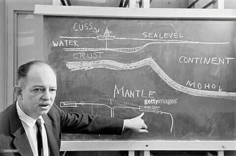
Image: Harry Hess with a blackboard

Image: USS Cape Johnson

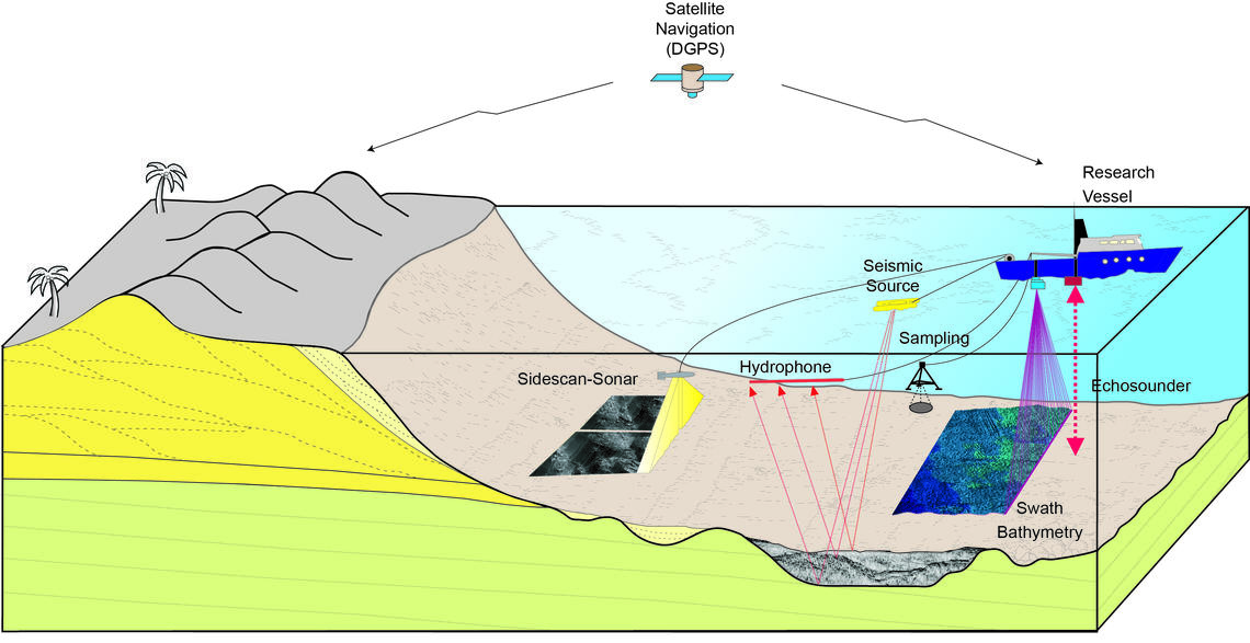
Modern methods to measure bathymetry include:

• Multi-beam echo sounders that map a wide swath of the seafloor.

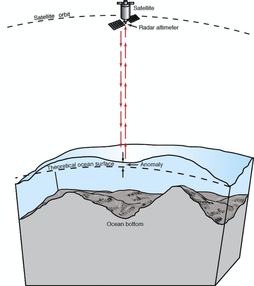
• Satellite measurement of variations in sea level due to variations in gravitational pull over bathymetric features – sea level is slightly lower over low spots on the sea floor and slightly higher over high spots.

Image: (left) Various methods of seafloor measurements made onboard a ship (right) Satellite measurements of variation in sea level due to variations in gravitational pull over bathymetric features.

import os
os.environ['PROJ_LIB'] = os.path.join(os.environ['CONDA_PREFIX'],'share/proj') # This is required for Basemap plotting to work

from mpl_toolkits.basemap import Basemap
import numpy as np
import matplotlib.pyplot as plt

fig = plt.figure(figsize=[14, 7])
# lon_0 is central longitude of projection.
# resolution = 'c' means use crude resolution coastlines.
m = Basemap(projection='robin',lon_0=0,resolution='c')
m.drawcoastlines()
# draw parallels and meridians.
m.drawparallels(np.arange(-90.,90.,30.))
m.drawmeridians(np.arange(-180.,180.,60.))
m.drawmapboundary()
m.etopo()
plt.title("Earth's Topography and Bathymetry",fontsize=20)
plt.show()

Clipping input data to the valid range for imshow with RGB data ([0..1] for floats or [0..255] for integers).

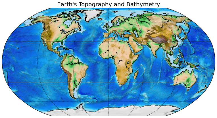
Image: topographic map of Earth

Mini-tutorial

• Opening netCDF files with xarray

• Making a topographic map

• Plotting a topographic cross-section

• Finding the maximum and minimum values in 2D data

We use ice sheet elevation from ETOPO1 Global Relief Model. In this tutorial, we will read a netCDF file using the XArray module and then make a topographic map of the United States and a cross-section across it. NetCDF (network Common Data Form) is a file format for storing multidimensional scientific data (variables) such as temperature, humidity, and pressure. Feel free to use the codes from this tutorial to plot the topography within region you are curious about.

Note: Plotting the entire Earth may cause the Python kernel to die! Hogs too much memory! If you want to look at the global map, please look at the image above or the physical map in the precept room.

import xarray as xr
import numpy as np
import matplotlib.pyplot as plt

# Read ETOPO1 topography data file
ds = xr.open_dataset('Files/ETOPO1_Ice_g_gmt4.grd')

# Display the content
ds

<xarray.Dataset>
Dimensions:  (x: 21601, y: 10801)
Coordinates:
  * x        (x) float64 -180.0 -180.0 -180.0 -179.9 ... 179.9 180.0 180.0 180.0
  * y        (y) float64 -90.0 -89.98 -89.97 -89.95 ... 89.95 89.97 89.98 90.0
Data variables:
    z        (y, x) float64 ...
Attributes:
    Conventions:  COARDS/CF-1.0
    title:        ETOPO1_Ice_g_gmt4.grd
    GMT_version:  4.4.0
    node_offset:  0

# Plotting the topographic map of the United States
# WARNING: Plotting the entire Earth may cause the kernel to die

min_lon = -130     # left-boarder of the map
max_lon = -60      # right-boarder of the map
min_lat = 20       # lower-boarder of the map
max_lat = 50       # upper-boarder of the map
fig = plt.figure(figsize=[9,5])
obj = ds.z.sel(x=slice(min_lon, max_lon),y=slice(min_lat, max_lat)).plot()
# a line representing the cross-section in the next figure
plt.plot([-125, -65], [37, 37], 'k')
plt.xlabel('Longitude', fontsize=12)
plt.ylabel('Latitude', fontsize=12)
plt.grid()

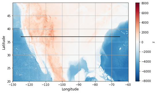
# Plotting a cross-section
plt.figure(figsize=[15,4])
ds_slice = ds.sel(y=37, method="nearest").sel(x=slice(-125,-65))
plt.plot(ds_slice['x'], ds_slice['z'], 'k', label='topography')
plt.plot([min(ds_slice['x']), max(ds_slice['x'])], [0, 0], 'c', label='sea level')
plt.grid()
plt.xlabel('Lontitude (degrees)', fontsize = 12)
plt.ylabel('Elevation above sea level (m)', fontsize = 12)
plt.title('Topography cross-section', fontsize=14)
plt.legend()
plt.show()

/home/globalseismology/.conda/envs/fall2022-sef/lib/python3.9/site-packages/xarray/core/indexes.py:234: FutureWarning: Passing method to Float64Index.get_loc is deprecated and will raise in a future version. Use index.get_indexer([item], method=...) instead.
  indexer = self.index.get_loc(

# Here is an example on how to determine the location of the highest and lowest points in the United States map
# Don't be surprised when you notice that the lowest point is outside the US
ds_usa = ds.sel(x=slice(-130, -60),y=slice(20, 50))

# min/max elevation
ds_max = ds_usa.where(ds_usa==ds_usa.max(), drop=True).squeeze()
ds_min = ds_usa.where(ds_usa==ds_usa.min(), drop=True).squeeze()

z_min = ds_min.z.data.item()
z_max = ds_max.z.data.item()

# finding the location of the min/max elevation point
lon_min = ds_min.x.data.item()
lat_min = ds_min.y.data.item()
lon_max = ds_max.x.data.item()
lat_max = ds_max.y.data.item()

print("The lowest point is at (lon, lat) = (%.2f, %.2f) and %.2f m below sea level."%(lon_min, lat_min, abs(z_min) ))
print("The highest point is at (lon, lat) = (%.2f, %.2f) and %.2f m above sea level."%(lon_max, lat_max, z_max))

The lowest point is at (lon, lat) = (-65.45, 20.00) and 8081.00 m below sea level.
The highest point is at (lon, lat) = (-121.77, 46.85) and 4161.00 m above sea level.

TO DO

Question 1 Checkout the topographic map above and focus on the Atlantic Ocean between North/South America and Eurasia/Africa using the tools discussed above. Note that the deepest part is not in the middle; instead there is an underwater mountain range that runs down the middle of the ocean. This is termed an ocean ridge or spreading ridge (more on spreading later). Note that while the ridge is a topographic high, it also has a valley (the “rift valley”) in the middle. Also look at the ocean ridges in the Indian, Pacific and Southern Oceans.

About how high does the mid-Atlantic ridge rise above the deep part of the Atlantic Ocean floor? Please make a cross-section plot of the bathymetry building on the tools provided above.

Answer:

Question 2 A “mid-ocean” ridge isn’t always in the middle of the ocean. Describe the position of the ridge in the Pacific Ocean called the “East Pacific Rise.” Please include a cross-section plot of the relevant portion of the Pacific Ocean to support the description.

Answer:

Question 3 Where is the only place where a “mid-ocean” ridge rises above sea level (hint, follow the mid-Atlantic ridge northwards)?

Answer:

Question 4 If the Earth’s lowest spots aren’t in the middle of the ocean, where are they? Focus on the west coast of South America and note the deep linear ocean trench about 100km off shore that runs along the length of the continent. Describe the locations of two other trench systems.

Answer:

Question 5 Where is the lowest point on Earth’s seafloor and the highest point on Earth’s land surface? What are the elevations of those points? Which is greater, the elevation of Mt. Everest above sea level or the depth of Challenger Depth below sea level. By how much in absolute and percentage terms? Does this surprise you?

Note: You will have to focus on both regions with Xarray and then use the tools above to get the range of values. Working with the full global data will likely throw an error!

Answer:

---

Part II: Seismicity

An earthquake is a vibration of Earth caused by the sudden release of energy, usually as an abrupt breaking of rock along planar fractures called faults. An earthquake initiates at its hypocenter or focus at some depth below the land surface or sea floor. The epicenter of the earthquake is defined as the point on the Earth’s surface above where the earthquake initiated.

But only rocks that are relatively cold and brittle (the Earth’s lithosphere) can be broken in earthquakes. Rocks that are hot and ductile (e.g. the Earth’s asthenosphere) will deform without breaking, and therefore do not produce earthquakes. By observing where earthquakes occur, both horizontally and with depth, we can learn where stress is concentrated and infer the material properties of the Earth.

In this section, we will examine the distribution of earthquakes. You will notice that most of them are near plate boundaries. Each type of plate boundaries has a unique moving pattern shown in the image below. Keep this in mind when you look at the earthquake epicenter plot later in this section.

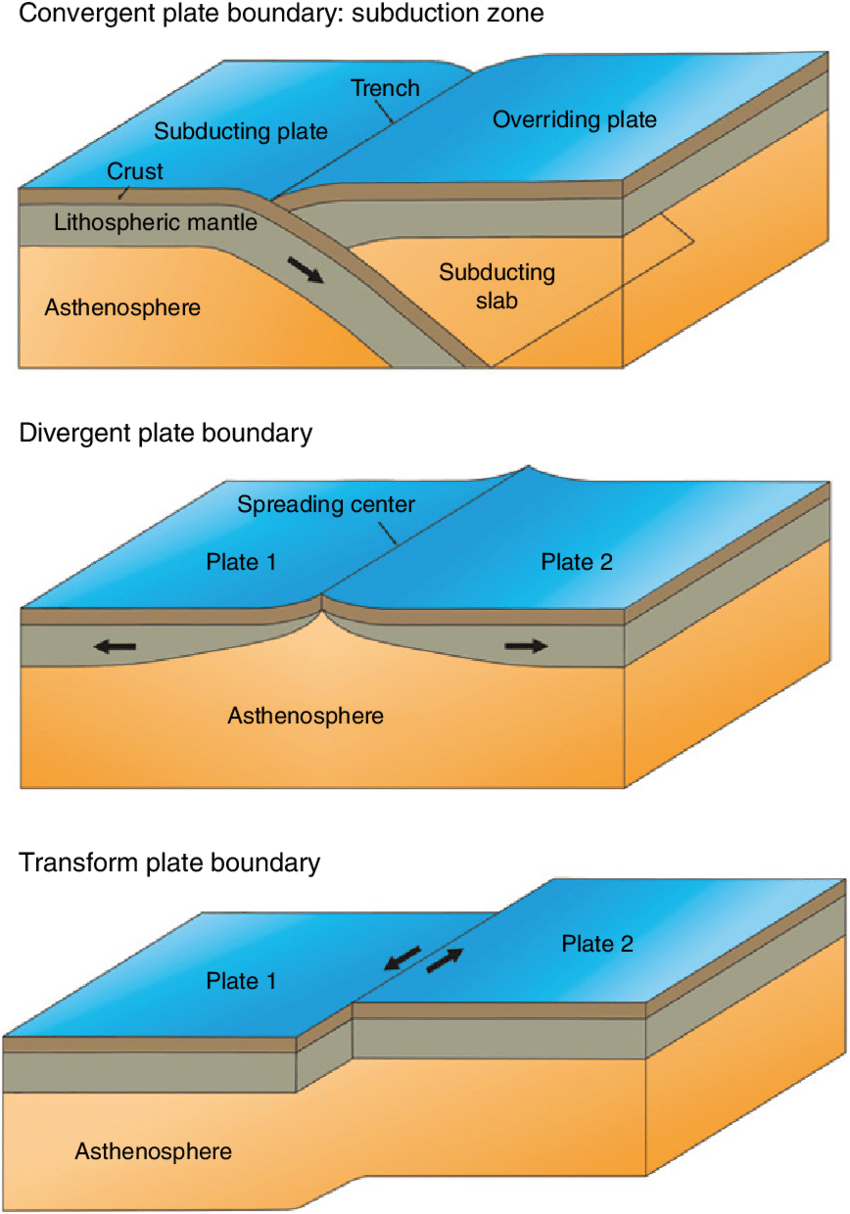
Image: Three major types of plate boundaries.

import pandas as pd
import json
import numpy as np
import plotly.express as px
import plotly.graph_objects as go

def cutoff_track(lon, lat, cutoff_lon):
    """
    Insert nan between two points that cross the cutoff lontitude. 
    Avoid horizontal line when plot the track
    
    Input Parameters:
    ----------------
    
    lon: longitude array
    lat: latitude array
    cutoff_lon: divide the curve at this cutoff longitude
    
    Return:
    ------
    
    lon, lat: updated arrays
    """
    xtrk = np.mod(lon - cutoff_lon, 360)
    is_cross = np.where(np.abs(xtrk[1:-1]-xtrk[0:-2]) > 90)[0]
    nans = np.empty(np.size(is_cross))
    nans[:] = np.nan
    lon = np.insert(lon, is_cross+1, nans)
    lat = np.insert(lat, is_cross+1, nans)
    return lon, lat

def load_plate_boundaries(filename):
    """
    Input Parameters:
    ----------------
    
    filename: input JSON file name containing the curve locations
    """    

    # Opening JSON file
    f = open(filename)

    # returns JSON object as a dictionary
    boundary = json.load(f)
    
    f.close()

    boundary = np.array(boundary[1])
    lons = boundary[:,0]
    lats = boundary[:,1]

    lons, lats = cutoff_track(lons, lats, 180)
    
    return lons, lats


def plot_earthquake_map(catalog):
    """
    Input Parameters:
    ----------------
    
    catalog: dataframe containing earthquakes
    """   
    
    rlons, rlats = load_plate_boundaries('Files/ridge.json')
    tlons, tlats = load_plate_boundaries('Files/transform.json')
    hlons, hlats = load_plate_boundaries('Files/trench.json')

    
    fig1 = px.scatter_geo(catalog, lon="ep.lon", lat="ep.lat", size="centroid.MW", color="ep.depth", 
                     labels={"ep.lon":"longitude (degrees)", "ep.lat":"latitude (degrees)", "centroid.MW":"Moment Magnitude",
                             "ep.depth":"depth (km)", "ep.timestamp":"origin time"}, 
                     hover_data=['ep.timestamp'])

    fig1a = px.line_geo(lon=rlons, lat=rlats)
    fig1a.update_traces(line={'color':'skyblue', 'width':3})
    
    fig1b = px.line_geo(lon=tlons, lat=tlats)
    fig1b.update_traces(line={'color':'lime', 'width':3})
    
    fig1c = px.line_geo(lon=hlons, lat=hlats)
    fig1c.update_traces(line={'color':'orangered', 'width':3})
    
    fig = go.Figure(data=fig1.data + fig1a.data + fig1b.data + fig1c.data, layout = fig1.layout)
    fig.update_xaxes(range=[-180, 180], tickvals=np.arange(-180,190,30))
    fig.update_yaxes(range=[-90, 90], tickvals=np.arange(-90,100,15))
    fig.update_geos(projection_type="robinson", lataxis_showgrid=True, lonaxis_showgrid=True)
    fig.update_layout(title_text="Global CMT catalog (N = %d earthquakes)"%len(catalog), title_x=0.5)
    fig.show()

# Read earthquake catalog
cmt_cat = pd.read_table("Files/Global_CMT_1972_2018.csv", delimiter=',')
cmt_cat = cmt_cat.sort_values(by=['ep.depth', 'centroid.MW'])

/tmp/ipykernel_130204/1742011327.py:2: DtypeWarning: Columns (15) have mixed types. Specify dtype option on import or set low_memory=False.
  cmt_cat = pd.read_table("Files/Global_CMT_1972_2018.csv", delimiter=',')

Review

Feel free to adjust the filter parameters in the cell below to have more or less earthquakes on the map. You may hover the dots to get the information of the earthquakes. The colors of the lines indicate the type of plate boundaries: Red is a Trench, Green is a Transform, and Blue is a Ridge boundary.

# Filter to improve readablility
Mw_min    = 6.5                               # Moment magnitude
Mw_max    = 10                                # Moment magnitude
depth_min = 0                                 # minimum depth in km
depth_max = 6400                              # maximum depth in km
datetime_min = '1000-01-01 00:00:00.000000'   # 'yyyy-mm-dd hh:mm:ss.SSSSSS'
datetime_max = '2050-01-01 00:00:00.000000'   # 'yyyy-mm-dd hh:mm:ss.SSSSSS'

# Don't change these two statements
mask = (cmt_cat['centroid.MW'] >= Mw_min) & (cmt_cat['centroid.MW'] <= Mw_max) & (cmt_cat['ep.depth'] >= depth_min) & (cmt_cat['ep.depth'] <= depth_max) & (cmt_cat['ep.timestamp'] >= datetime_min) & (cmt_cat['ep.timestamp'] <= datetime_max)
plot_earthquake_map(cmt_cat[mask])

/tmp/ipykernel_130204/2441878313.py:18: RuntimeWarning: invalid value encountered in remainder
  xtrk = np.mod(lon - cutoff_lon, 360)

TO DO

Question 6. Examine the regions on and around Earth’s ocean ridges and ocean trenches. Both the spatial distribution and the depths of earthquakes associated with each are different. Describe/illustrate these differences between earthquake associated with ridges and earthquakes associated with trenches.

Answer:

Question 7. Using earthquake depths as evidence, discuss whether the Earth’s lithosphere is thicker at ridges or at trenches.

Answer:

Question 8. Consider the belt of deepest earthquakes parallel to the Andes mountain chain (the 150-800km deep earthquakes). On what plate are these earthquakes? Explain.

Answer:

---

Part III: Volcanism

A volcano is an opening in the Earth’s surface through which melted rock (magma), volcanic ash and/or gases escape from the interior of the Earth. Most of these are on land, but some are underwater (called “seamounts”). Hovering on a particular volcano icon brings up an information box about that volcano. Hover over the dots in the interactive plot below to check out the primary volcano type (also see legend) and the last known eruption.

Mid-ocean ridge volcanism: While the volcano map below shows more than 1500 volcanoes, the vast majority of volcanic activity on Earth does not occur on land nor does it build volcanoes; instead it occurs at fissures underwater along the mid-ocean ridge system.

# Use encoding='cp1252' to avoid UnicodeDecodeError: 'utf-8' codec can't decode byte 0x92
# in position 87438: invalid start byte
# See this https://stackoverflow.com/questions/29419322/unicodedecodeerror-utf8-codec-cant-decode-byte-0x92-in-position-377826-inva
volcanoes = pd.read_csv("Files/GVP_Volcano_List_Holocene.csv", encoding='cp1252')

# Dissplay the content of the dataframe
volcanoes[['Volcano Name', 'Primary Volcano Type', 'Last Known Eruption', 'Country', 'Tectonic Setting','Dominant Rock Type']]

	Volcano Name	Primary Volcano Type	Last Known Eruption	Country	Tectonic Setting	Dominant Rock Type
0	West Eifel Volcanic Field	Maar	8300 BCE	Germany	Rift zone / Continental crust (>25 km)	Foidite
1	Chaine des Puys	Lava dome	4040 BCE	France	Rift zone / Continental crust (>25 km)	Basalt / Picro-Basalt
2	Olot Volcanic Field	Pyroclastic cone	Unknown	Spain	Intraplate / Continental crust (>25 km)	Trachybasalt / Tephrite Basanite
3	Calatrava Volcanic Field	Pyroclastic cone	3600 BCE	Spain	Intraplate / Continental crust (>25 km)	Basalt / Picro-Basalt
4	Colli Albani	Caldera	Unknown	Italy	Subduction zone / Continental crust (>25 km)	Foidite
...	...	...	...	...	...	...
1327	Leskov Island	Stratovolcano	Unknown	United Kingdom	Subduction zone / Oceanic crust (< 15 km)	Andesite / Basaltic Andesite
1328	Zavodovski	Stratovolcano	2016 CE	United Kingdom	Subduction zone / Oceanic crust (< 15 km)	Basalt / Picro-Basalt
1329	Protector Seamounts	Submarine	1962 CE	United Kingdom	Subduction zone / Oceanic crust (< 15 km)	Rhyolite
1330	Mount Haddington Volcanic Field	Shield	Unknown	Antarctica	Intraplate / Continental crust (>25 km)	Basalt / Picro-Basalt
1331	Melville	Stratovolcano	Unknown	Antarctica	Intraplate / Continental crust (>25 km)	NaN

1332 rows × 6 columns

rlons, rlats = load_plate_boundaries('Files/ridge.json')
tlons, tlats = load_plate_boundaries('Files/transform.json')
hlons, hlats = load_plate_boundaries('Files/trench.json')
    
fig1 = px.scatter_geo(volcanoes, lon="Longitude", lat="Latitude", color='Primary Volcano Type', 
                 symbol_sequence=['triangle-up'],
                 labels={"Longitude":"longitude (degrees)", "Latitude":"latitude (degrees)","color":"Last Known Eruption (years before present)"}, 
                 hover_data=['Volcano Name', 'Primary Volcano Type', 'Last Known Eruption', 'Country', 'Tectonic Setting','Dominant Rock Type'])

fig1a = px.line_geo(lon=rlons, lat=rlats)
fig1a.update_traces(line={'color':'skyblue', 'width':3})
    
fig1b = px.line_geo(lon=tlons, lat=tlats)
fig1b.update_traces(line={'color':'lime', 'width':3})
    
fig1c = px.line_geo(lon=hlons, lat=hlats)
fig1c.update_traces(line={'color':'orangered', 'width':3})

fig = go.Figure(data=fig1a.data + fig1b.data + fig1c.data + fig1.data, layout = fig1.layout)

fig.update_xaxes(range=[-180, 180], tickvals=np.arange(-180,190,30))
fig.update_yaxes(range=[-90, 90], tickvals=np.arange(-90,100,15))
fig.update_traces(marker={'size': 15})
fig.update_geos(projection_type="robinson", lataxis_showgrid=True, lonaxis_showgrid=True)
fig.update_layout(title_text="Active Volcanoes (N = %d)"%len(volcanoes), title_x=0.5)
fig.show()

/tmp/ipykernel_130204/2441878313.py:18: RuntimeWarning:

invalid value encountered in remainder

TO DO

Question 9. You have seen that earthquakes are associated with plate boundaries, and we mention above that volcanism exists along the mid-ocean ridges. What about volcanism associated with trenches? Describe the spatial distribution of volcanoes associated with trenches and surrounding features (e.g. coastlines, island arcs, mountain ranges).

Answer: