Geophysical Field Survey

IN THE SPACE BELOW, WRITE OUT IN FULL AND THEN SIGN THE HONOR PLEDGE:

“I pledge my honor that I have not violated the honor code during this examination.”

PRINT NAME:

If a fellow student has contributed significantly to this work, please acknowledge them here:

Peer(s):

Contribution:

By uploading this assignment through Canvas, I sign off on the document below electronically.

---

Modern Geoscience uses a multitude of observations to make inferences about the Earth’s past, present and future. Historically, observations in Geology were limited to surface observations such as fossil assemblages and rock formations. Students of geology develop skills to visualize the process within the Earth from the obervations. Modern Physics is a branch of study focused on describing various phenomena by formulation of mathematical expressions, often translated to computer code (such as the ones in this course!) for efficient calculations. Applying both visualization and mathematical formulation to study the Earth gives rise to geophysics. Geophysics is the application of the methods of physics to the study of the Earth. Geophysics ‘sees’ the Earth in terms of its physical properties such as density, which complement and often validate the usual types of geological information.

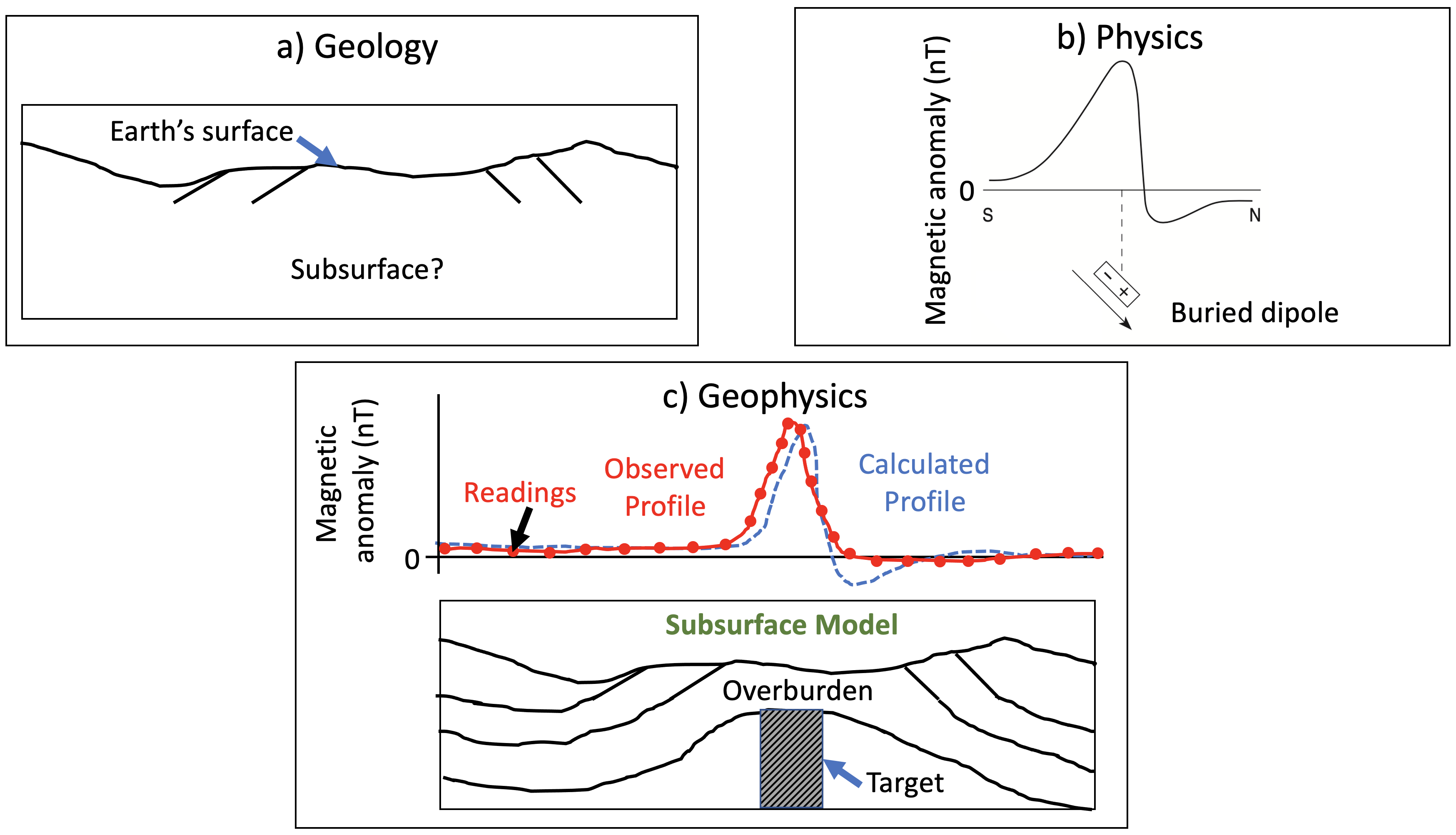
Figure: (a) A cross-section illustrating surface geology with no subsurface information. (b) Model of physical parameter. The presence of a burial magnetic dipole cause the magnetic field anomaly observed on the surface. © Observed the magnetic anomaly along with a model of subsurface magnetic susceptibility that might cause such a change. The model agrees with the observed surface geology.

Borehole drilling is the only way to directly measure the physical properties of rocks. However such artifical, invasive procesures are expensive and damage the environment. Nevertheless, they are sometimes done to a depth of few hundred feet before construction of major projects (e.g. geothermal plant at Princeton) or for understanding regional stratigraphy. These barely scratch the skin of the Earth, which has an average radius of 6371 km. Kola Superdeep Borehole SG-3 retains the world record at 12.262 km (40,230 ft) reached in 1989 and is still the deepest artificial point on Earth. Borehole drilling has only been done at a few locations. Therefore, our vast understanding of the Earth’s inner workings comes from geophysical measurements made from the Earth’s surface or through remote sensing from orbiting satellites. We will focus on the geophysical measurements that can be made by human beings on land using different kinds of instruments (Table 1). A field survey is the method of collecting data for making inferences about the physical properties of the Earth’s interior.

Instrument	LaCoste and Romberg Gravimeter	Superconducting Gravimeter	Accelerometer	Broadband Seismometer	Magnetometer	GPS	Radar
Property Measured at the Earth’s Surface	gravitational acceleration	gravitational acceleration	acceleration	ground motion	magnetic field intensity	position	electro-magnetic field
Property Investigated within Earth	density	density	seismic velocity, density, and attenuation	seismic velocity, density, and attenuation	magnetic susceptibility and remanent magnetization	density, viscosity	electrical conductivity
Governing Equation	Newton law of gravity	Newton law of gravity	Wave equation	Wave equation	Maxwell’s Equations	General Relativity	Maxwell’s Equations
Frequency Range	0-1 Hz	0-1 Hz	0-100 Hz	0.001-100 Hz	< 100 Hz	< 1 Hz	25-1000 MHz

Table 1: comparison of geophysical instruments on measured quantities, governing equation, and working frequency ranges. A frequency of 0 Hz means the instrument can measure a value at the steady-state.

Geophysical signals exist in a variety of forms, ranging from natural sources (e.g. mineral deposits) to anthropogenic noise (e.g. cars on a road), and manifest themselves as changes in various properties. These signals can vary either in their pattern or strength/amplitude depending on the time and location of measurement. For instance, the magnetic field at any location on Earth changes with time and we may want to record this temporal variation to understand the geodynamo in the core that creates this field. Alternatively, a buried drum or pipe may have a magnetic field that varies with location, which would be of interest to a civil and environmental engineer. Several categories of geophysical signals can indeed vary both with time and location. Seismic and ground penetrating radar signals fall into this category; these signals inform our understanding of both the current state and evolution of physical properties in the subsurface.

An important aspect of the variation in geophysical signals pertains to its wavelength in time or space (\(T\)), and its inverse, frequency (\(f\) = 1/\(T\)). As we shall see, various sources of signals manifest at different frequencies. For example, a shallow and small metallic object buried a few meters deep might give rise to high-frequency signals localized in space. On the other hand, a subducting slab that is a few hundreds of meters wide will give rise to signals that are longer in spatial wavelength (or lower in spatial frequency). One can also think of frequency range of geophysical signals; a transient vibration from a local earthquake will be high in its temporal frequency but deformation in the solid Earth due to tides will operate at lower frequencies. Depending on what the signal of interest, a decision about the primary geophysical instrument is made by the practitioner (Table 1).

Part I: Geophysical Instruments

Here is a summary of various intruments that are widely used in a geophysical survey. Gravimeters probe the gravity field, seismometers probe the ground movement, magnetometer probe the magnetic field, and ground penetrating radar can infer the burried structure.

Gravimeter

A gravimeter is a sensitive instrument that can measure differences much less than a millionth of the surface gravity, \(g\). This measurement can be done in three major ways. One way is to time the fall of an object, though this can be done very accurately in the laboratory but is rather inconvenient for measurements in the field. A second way is to use a pendulum, since its period depends upon the value of \(g\) as well as its dimensions. This has been used widely in the past, but requires a bulky apparatus and takes considerable time. It has been largely superseded by the third way, which uses a spring balance, shown schematically in Figure 2. The pull of gravity on the mass, \(m\), extends the spring, so that the spring has a slightly greater extension at places where \(g\) is larger. A spring balance measures the weight of a body, the pull of gravity upon its mass, \(m\), equal to \(mg\). In contrast, a pair of scales compares masses, and if two masses are equal they will balance everywhere. Thus the mass of \(m\) is constant but its weight varies from place to place, as we know from the near-weightlessness of objects in space.

Modern gravity meters or gravimeters can detect changes in \(g\) as small as a hundredth of a mGal or about 10\(^{\text{–8}} g\), and some extra-sensitive instruments can do considerably better. Such differences are much smaller than those measured in other branches of geophysics, so a gravimeter is an instrument of choice for many applications. To take a reading, the instrument is accurately levelled on a firm surface, and if it has a thermostat (to prevent the length of the spring varying due to internal temperature changes), the temperature is checked. Next, the mass is restored to a standard position by means of a screw and the number of turns of the screw is the reading. A practised operator can carry out the whole operation in a few minutes. Some instruments are fitted with electronic readouts that provide a number that can be fed into a computer, ready for data processing.

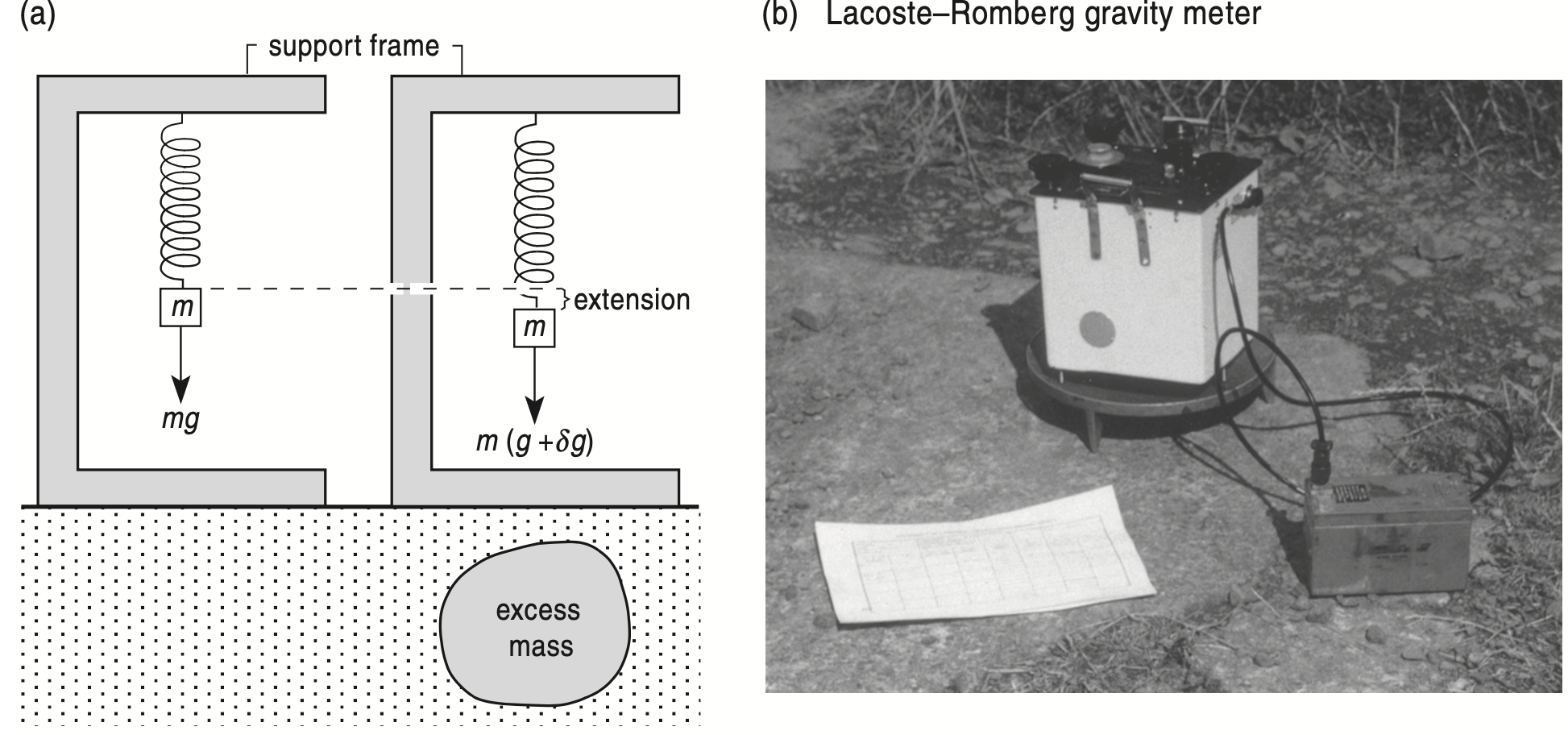
Figure: Gravimeters need careful handling and are usually transported inside a protective box. Source: Looking Into the Earth: An Introduction to Geological Geophysics

LaCoste and Romberg Gravimeter

LaCoste and Romberg gravimeters rely on a mass, supported by some kind of spring, responding to the pull of the Earth’s gravity. Because the changes to be measured are so small, the spring is arranged to amplify the effect (Figure below). Initially, the beam is at rest in position (i), with the pull of the spring balancing the pull of gravity on the mass. When the gravimeter is moved to where g is larger, the beam rotates to a new balance (ii), where the extra pull of the extended spring balances the extra pull of gravity.

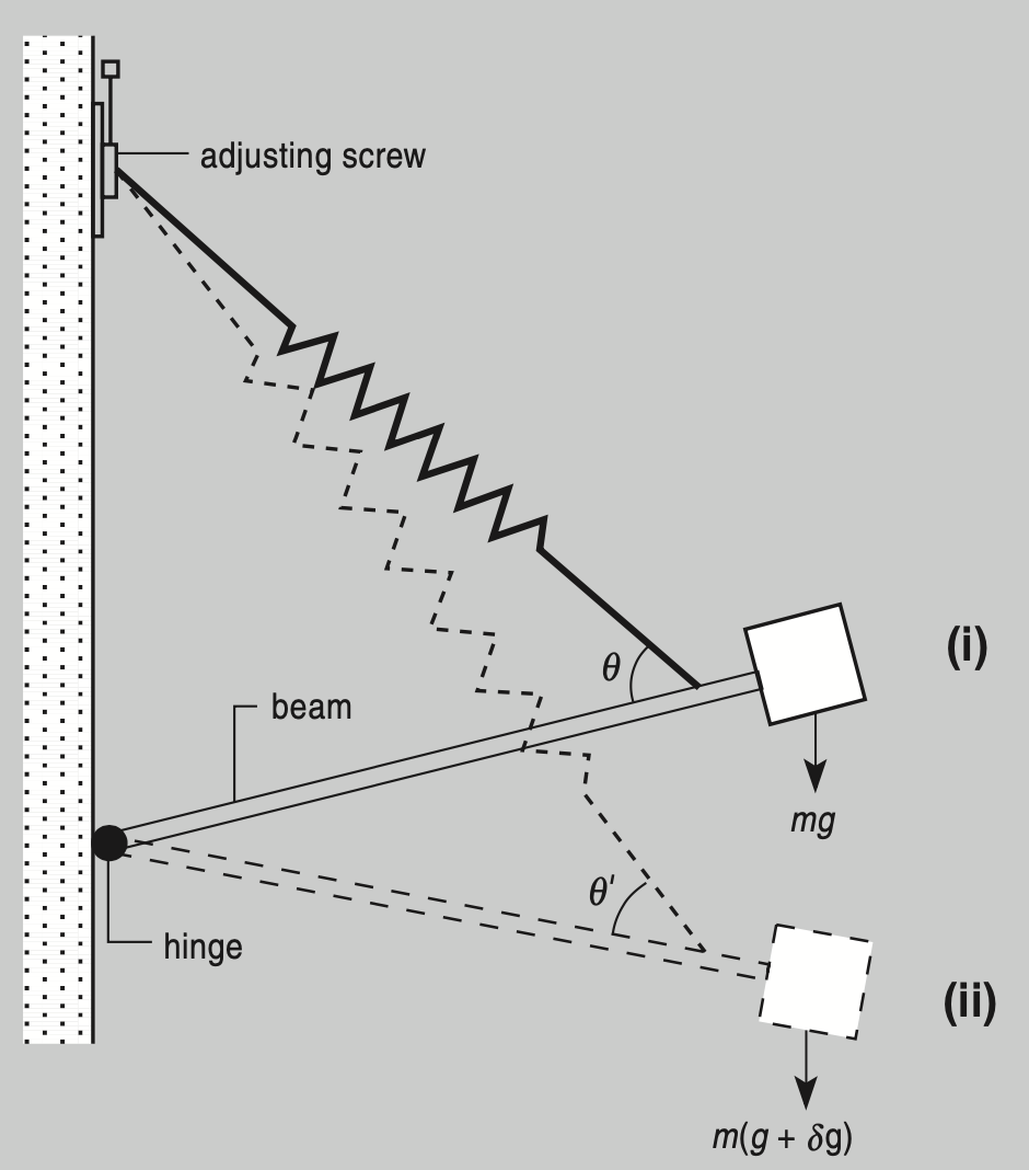
Figure: LaCoste and Romberg Gravimeter. Source: Looking Into the Earth: An Introduction to Geological Geophysics

Superconducting Gravimeter

Other relative gravimeters and seismometers are based on a test mass that is suspended by a spring attached to the instrument support. A change in gravity or motion of the ground moves the test mass and this motion generates a voltage that becomes the output signal (velocity or acceleration). Even in a thermally well-regulated environment the mechanical aspects of a spring suspension causes erratic drift that is difficult to remove by post processing. The superconducting gravimeter solves the drift problem by replacing the mechanical spring with the levitation of a test mass using a magnetic suspension.

The levitation force is produced by the interaction between the magnetic field from the coils and the currents induced on the surface of the superconducting sphere. The current in the coils can be precisely adjusted to balance the force of gravity on the sphere at the center of the displacement transducer. As a result, a very small change in gravity (acceleration) gives a large displacement of the test mass. This allows for the instrument to achieve very high sensitivity. Because the levitation is magnetic, changes in the Earth’s magnetic field would seriously degrade its stability. A superconducting shield is used to exclude the earth’s magnetic field from entering the space where the sensor is housed.

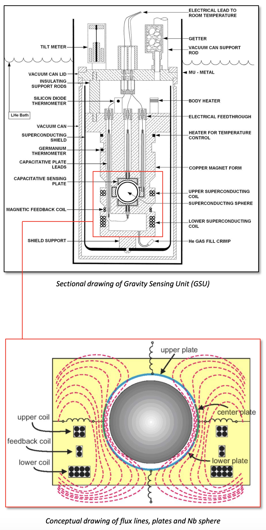
Figure: The inner workings of a superconducting gravimeter. Source: Operating Principles of the Superconducting Gravity Meter

Seismometer

Seismometers record ground motions ranging from large high-frequency accelerations near an earthquake to small ultra-long-period normal mode signals. Because no single seismograph can do this, different instruments have evolved to handle different dynamic ranges (amplitude) and frequency ranges of seismic waves.

Accelerometer

An accelerometer is a type of inertial sensor which is configured to detect accelerations down to zero frequency. Unlike a gravimeter, they are typically configured to read peak accelerations on the order of 1 \(g\) or larger without clipping and thus must have relatively low sensitivities. They can be used to detect static accelerations, for the purpose of integrating them to obtain position as in an inertial guidance system, or they can be used to detect strong seismic motions. Like a gravimeter they have a flat response to acceleration down to zero frequency, but the upper corner of their low-pass response will be at a much higher frequency.

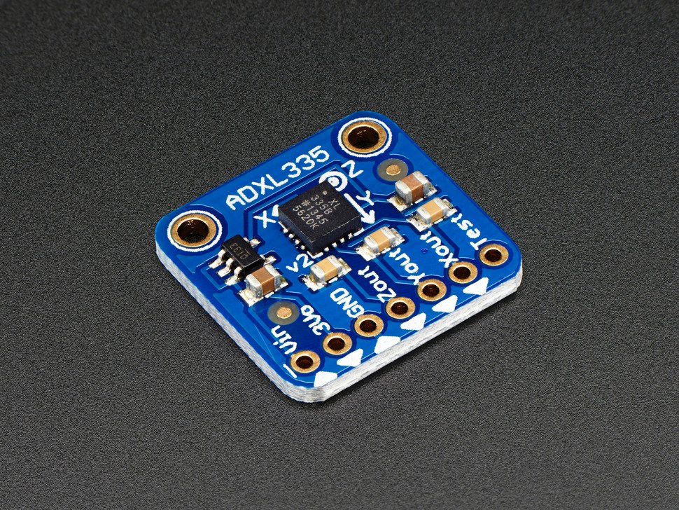
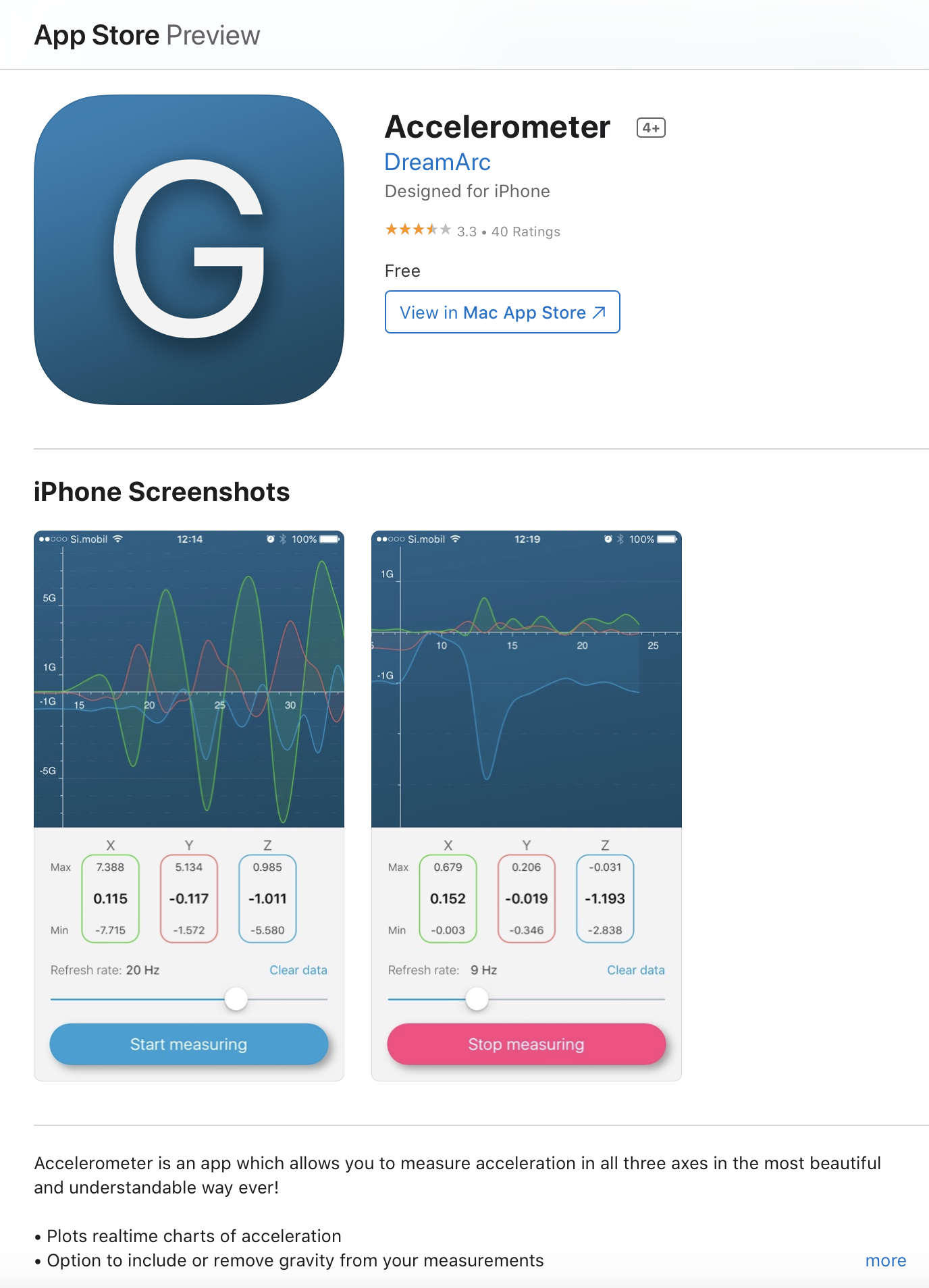
Figure: (left) Accelerometer chip (right) An example of accelerometer application. Source: Adafruit and Apple App Store.

Broadband seismometer

A broadband seismometer can record a very broad frequency range (0.001-100 Hz) but not down to zero frequency of ground motion: displacement, velocity, or acceleration. It has a higher sensitivity and therefore measures much smaller motions than an accelerometer.

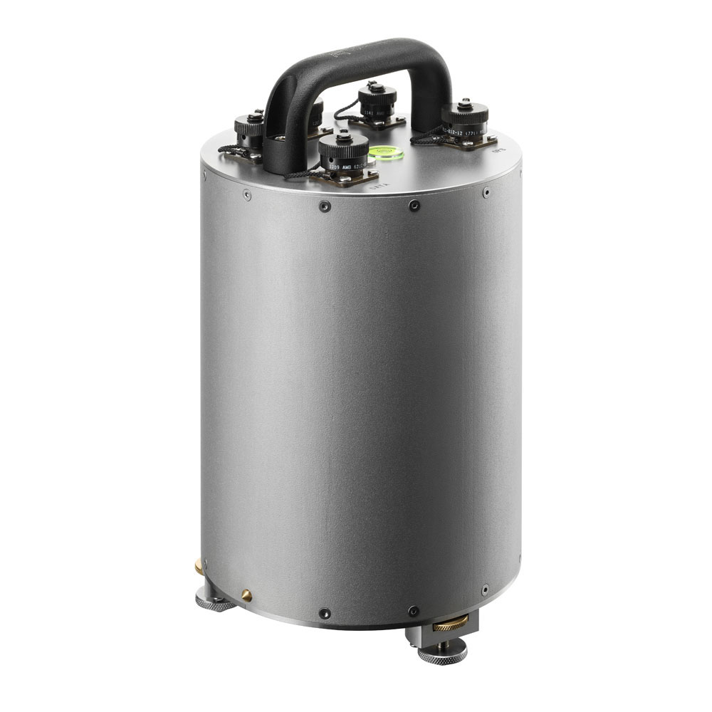
Figure: a broadband seismometer. Source: essearth.com

GPS

GPS is fully operational and meets the criteria established in the 1960s for an optimum positioning system. The system provides accurate, continuous, world-wide, three-dimensional position and velocity information to users with the appropriate receiving equipment. GPS also disseminates a form of Coordinated Universal Time (UTC). The satellite constellation nominally consists of 24 satellites arranged in 6 orbital planes with 4 satellites per plane. The system utilizes the concept of one-way time of arrival (TOA) ranging. Satellite transmissions are referenced to highly accurate atomic frequency standards onboard the satellites, which are in synchronism with a GPS time base. This technique requires that the user receiver also contain a clock. Utilizing this technique to measure the receiver’s three-dimensional location requires that TOA ranging measurements be made to four satellites. If the receiver clock were synchronized with the satellite clocks, only three range measurements would be required. However, a crystal clock is usually employed in navigation receivers to minimize the cost, complexity, and size of the receiver. Thus, four measurements are required to determine user latitude, longitude, height, and receiver clock offset from internal system time. If either system time or height is accurately known, less than four satellites are required.

Ground Penetrating Radar (GPR)

Ground-penetrating radar, GPR, has by far the highest frequency of any electro-magnetic method and displays the wave aspect most clearly. It depends on reflection of pulses of waves, and so resembles seismic reflection. A pulse of electro-magnetic waves is transmitted downwards, reflects off interfaces, and is received back at the surface and the reflection time (two-way time, TWT) is used as a measure of the distance to the target. The transmitter has an antenna (or aerial), producing an extremely short pulse of waves, lasting only a few nanoseconds (a nanosecond, ns, is a thousandth of a millionth, or 10\(^{–9}\), seconds). These pulses contain frequencies in the range 25 to 1000 MHz, and the shorter the pulse the higher its frequency. Such short pulses are needed because electro-magnetic waves travel so fast that the TWTs, for interfaces that may be less than a meter deep, are extremely small.

GPR is increasingly used in situations where its high resolution is a great advantage, and its limited penetration is sufficient. Uses include hydrogeology (particularly for finding the position of the water table), environmental geophysical surveying (polluted ground), site engineering (faulting, fractures, cavities, and buried metal structures), mineral exploration, and archaeology. It can also be used for mapping Quaternary soils, such as showing the structure of fluvial sediments, or to investigate the detailed structures of oil reservoir rocks, including its use in boreholes.

Magnetometer

Magnetometers used for magnetic surveying differ from the types used to measure the magnetisation of rock samples in the laboratory because they need to measure the strength of the field rather than the strength of magnetisation of a sample, and they have to be portable. There are two main types. The proton precession magnetometer, usually abbreviated to proton magnetometer measures the total strength of the magnetic field but not its direction and so shows a total field anomaly (also called a total intensity anomaly), while the fluxgate magnetometer measures the component of the field along the axis of the sensor; for land surveying the sensor is usually aligned vertically for this is easy to do, giving a vertical component anomaly, but in aircraft, ships, and satellites it is kept aligned along the field and so measures the total field and also gives its direction. The sensor of a proton precession magnetometer need not be oriented (except roughly), and its readings do not ‘drift’ with time, in contrast to that of a fluxgate magnetometer, which has to be kept aligned and does drift. However, proton precession magnetometers take a few seconds to make a reading and are best kept stationary while this is being done, whereas fluxgates give a continuous reading, which can result in quicker surveying when readings are taken at short intervals. Both types can measure the field to 1 nT or less, which is more than sufficient for most anomalies. In practice, proton magnetometers are used for most ground surveys, except that fluxgates are usually chosen for detailed gradiometer surveys and in boreholes, for a variety of reasons. Both types are used in aerial surveys. A third type, the caesium vapor magnetometer, is more expensive but is sometimes used when higher sensitivity is needed. Caesium vapor oscillates continuously in the presence of the ambient magnetic field. The frequency of oscillation is proportional to the ambient magnetic field. Modern magnetic processors have a resolution of 0.001 nT and read 10 times each second or faster.

Magnetic surveying can be carried out on the ground, from aircraft, and from ships. Commonly used instruments are the proton (precession) magnetometer, which measures the total field, and the fluxgate magnetometer, which measures a component of the field; for ground surveys this component is usually the vertical one, but in ships and aircraft it is along the field and so effectively measures the total field and its direction. Gradiometers use a pair of sensors, usually fluxgates.

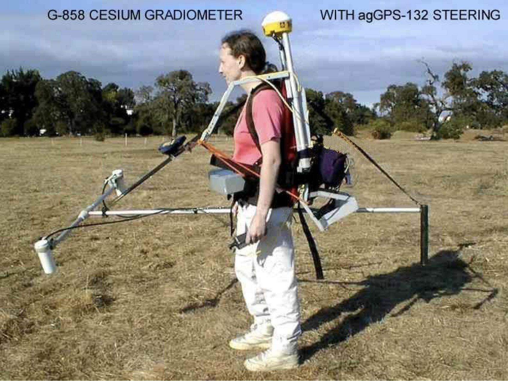
Figure: A caesium vapor magnetometer. Source: Geometrics

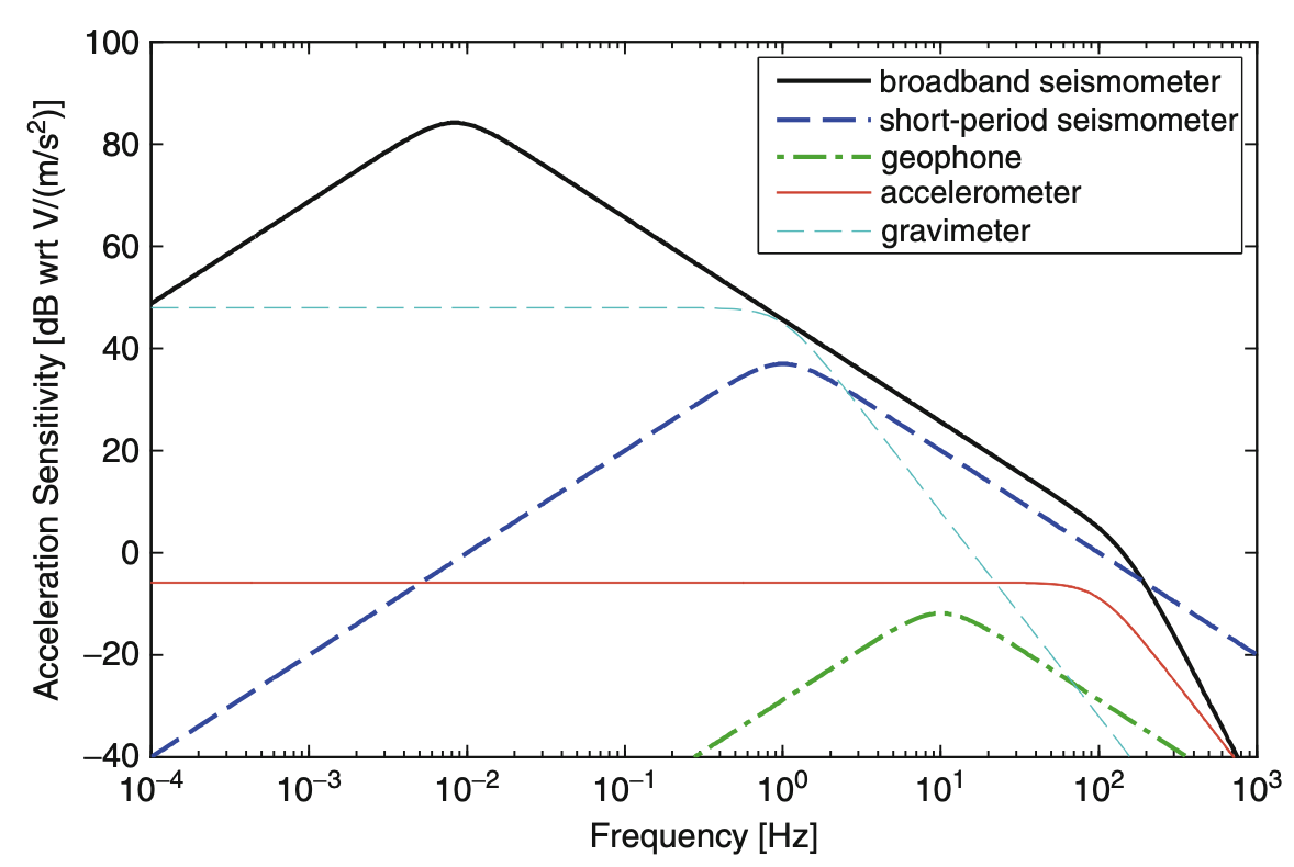
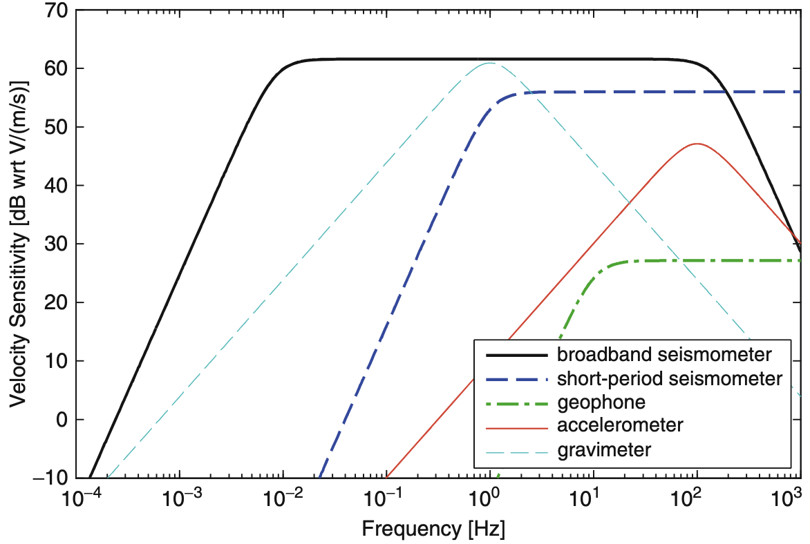
Figure: The frequency ranges depends on the sensitivity of the instruments at any given frequency. Source: Principles of Broadband Seismometry, Encyclopedia of Earthquake Engineering

Question 1 Comment on which instrument(s) would be appropriate for each of these applications. Assume that there is no budgetary limitation.

• Prospecting for gold

• Finding a skeleton

• Exploration of oil and gas

• Thickness of a glacier

• Monitor volcanic activity

Answer

---

Part II: Designing a Field Survey

Data acquisition

Most geophysical measurements are made at the Earth’s surface, either to save the expense and time of drilling, or because it is not feasible to go deep enough. Therefore the first actual step, after planning, to carry out a geophysical survey, is data acquisition, a set of measurements made with a geophysical instrument. Often the instrumental readings are taken along a line or traverse. Usually, readings are not taken continuously along the traverse but are taken at intervals, usually regular, and each place where a reading is taken is called a station. When the readings are plotted – often after calculations – they form a profile.

The presence of a target is often revealed by an anomaly. In everyday language an ‘anomaly’ is something out of the ordinary, but in geophysics it is very common, for an anomaly is simply that part of a profile, or contour map, that is above or below the surrounding average.

Signal and Noise

The profile may not reveal the presence of the target as clearly as one would like, because of noise, the unwanted variations or fluctuations in the quantities being measured. What is noise and signal may depend on the purpose of the survey; when searching for a weak magnetic anomaly of a granite intrusion the strong anomalies of basaltic dykes would be noise, whereas to a person looking for dykes they are the signal.

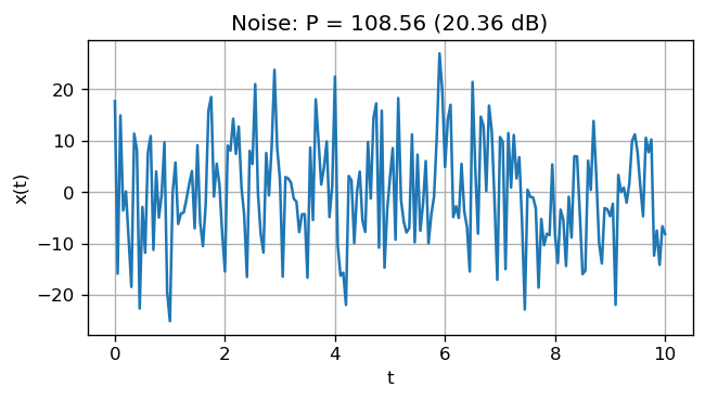
The noise level is charcterized by the power. The power of the noise is the variance of the noise: $\( P_{\text{noise}} = \frac{\sum_{i=1}^N (x_i - \bar{x})^2}{N - 1} \)\( The noise power can be represented in the logarithmic decibel (dB): \)\( P_{\text{noise, dB}} = 10 \log_{10} (P_{\text{noise}}) \)$

The figure shows an example of random noise. Each sample is drawn from a normal distribution with a population mean of 0 and a population variance of 100. You can see that the actual noise power is different from the variance of the distribution by a bit due to the nature of randomness.

import numpy as np
import matplotlib.pyplot as plt

# creating random noise: normal distribution, mean = 2, std = 1
t = np.linspace(0,10,201)
x_noise = 10 * np.random.normal(0,1,size=np.shape(t))

# noise level
P_noise = np.var(x_noise)
P_noise_dB = 10 * np.log10(P_noise)

plt.figure(figsize=[6,3], dpi=120)
plt.plot(t,x_noise)
plt.grid()
plt.xlabel('t')
plt.ylabel('x(t)')
plt.title('Noise: P = %.2f (%.2f dB)' % (P_noise, P_noise_dB))

plt.show()

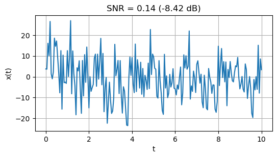
The noise level on its own may not indicate whether it is “loud” or not unless we have something to compare. The common way is to compare with the level of the signal. Such quantity is called the signal-to-noise ratio (SNR): $\( \text{SNR} = \frac{P_{\text{signal}}}{P_{\text{noise}}} = \frac{\text{Var} (x_{\text{signal}})}{\text{Var} (x_{\text{noise}})} \)\( and in decibel, \)\( \text{SNR}_{\text{dB}} = 10 \log_{10} (\text{SNR}) = P_{\text{signal, dB}} - P_{\text{noise, dB}} \)$

Here is an example of a sinusoidal signal with an amplitude of 50 with a random noise with a variance of 100.

t = np.linspace(0,10,201)
x_noise = 10 * np.random.normal(0,1,size=np.shape(t))

# noise level
P_noise = np.var(x_noise)
P_noise_dB = 10 * np.log10(P_noise)

# now add a sinusoidal wave with an amplitude of 5 (smaller than the noise)
x_signal =  50 * np.sin(2*np.pi/2*t)

# signal level
P_signal = np.var(x_signal)
P_signal_dB = 10 * np.log10(P_signal)

# SNR
snr = P_signal / P_noise
snr_dB = P_signal_dB - P_noise_dB

# the sum of signal and noise
x_all = x_signal + x_noise

plt.figure(figsize=[6,3], dpi=120)
plt.plot(t,x_all)
plt.grid()
plt.xlabel('t')
plt.ylabel('x(t)')
plt.title('SNR = %.2f (%.2f dB)' % (snr, snr_dB))
plt.show()

print('Signal : P = %.2f (%.2f dB)' % (P_signal, P_signal_dB))
print('Noise  : P = %.2f (%.2f dB)' % (P_noise, P_noise_dB))
print('SNR    :     %.2f (%.2f dB)' % (snr, snr_dB))

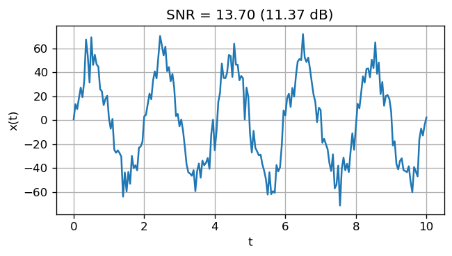
Signal : P = 1243.78 (30.95 dB)
Noise  : P = 90.81 (19.58 dB)
SNR    :     13.70 (11.37 dB)

Let’s look at an example of a sinusoidal signal with an amplitude of 5 embeded in a random noise with a variance of 100.

t = np.linspace(0,10,201)
x_noise = 10 * np.random.normal(0,1,size=np.shape(t))

# noise level
P_noise = np.var(x_noise)
P_noise_dB = 10 * np.log10(P_noise)

# now add a sinusoidal wave with an amplitude of 5 (smaller than the noise)
x_signal =  5 * np.sin(2*np.pi/2*t)

# signal level
P_signal = np.var(x_signal)
P_signal_dB = 10 * np.log10(P_signal)

# SNR
snr = P_signal / P_noise
snr_dB = P_signal_dB - P_noise_dB

# the sum of signal and noise
x_all = x_signal + x_noise

plt.figure(figsize=[6,3], dpi=120)
plt.plot(t,x_all)
plt.grid()
plt.xlabel('t')
plt.ylabel('x(t)')
plt.title('SNR = %.2f (%.2f dB)' % (snr, snr_dB))
plt.show()

print('Signal : P = %.2f (%.2f dB)' % (P_signal, P_signal_dB))
print('Noise  : P = %.2f (%.2f dB)' % (P_noise, P_noise_dB))
print('SNR    :     %.2f (%.2f dB)' % (snr, snr_dB))

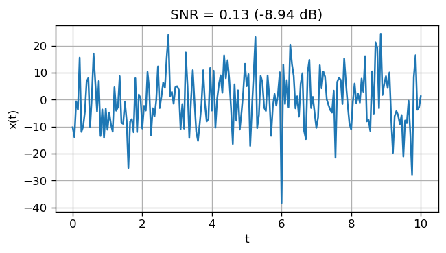
Signal : P = 12.44 (10.95 dB)
Noise  : P = 97.37 (19.88 dB)
SNR    :     0.13 (-8.94 dB)

Notice that the signal is not clear in this time-series data. As you can see, the signal-to-noise ratio is below 1. The general way to make the signal clearer is to use signal processing which will be discussed later on.

Modeling

A model in geophysical usage is a body or structure described by physical properties such as depth, size, density etc. that could account for the data measured. The model is almost always simpler than the actual Earth by several reasons. First, the observation is often blurred compared to the causative body. For example, the profile has extended tails to both sides while the target body has sharp edges. Second, the observations are taken at intervals not continuously. We can do our best by improving the resolution when it is possible. Third, the noise and the measurement errors make it difficult to determine the shape and size of anomaly. There are two main ways to determine the model from the observations. One way is deducing the model directly from the observations. This is called inverse modeling. On the other hand, we may need to guess the model and compare the predictions from the model with the observations, and then modify the model until the prictions match the observations. This process is called forward modeling.

Geological interpretation

Finally, the physical model has to be translated into geological terms; a large, roughly cylindrical mass with density less than its surroundings may be interpreted as a granite pluton; an elongated anomaly of low electrical resistance as a galena vein, and so on. This stage in the interpretation needs to take account of all available information, from the general geological context within which the survey was carried out, to information from outcrops, boreholes, and any other geophysical surveys. To neglect the other available information, either geophysical or geological, is like relying only on your hearing when you can see as well. Such information may allow you to choose between different physical models that match the geophysical observations.

Data processing

Even after the results of a survey have been acquired and displayed, the targets of interest may not be obvious. There may be a need for further stages of processing that will enhance the features. Signals in time or space are continuous. Consider the magnetic field, barometric pressure, ground motion, or wind speed at any location. Each of these quantities varies continually with time. Most instruments are electromechanical devices that produce a continuous waveform as a function of time. If this waveform were recorded directly then we would have an analogue signal. (e.g. a barometric pressure chart, ground motion measured with a pen on a rotating drum). Prior to the age of digital recorders analogue records were the only form of data collection. Today most signals are digitally sampled so they can be stored on computers, processed and plotted. Before looking at sampling we consider the simplest and most fundamental of all signals, sinusoids.

Harmonic analysis

Sinusoids can be written as:

\[ \sin \omega t, \cos \omega t, \sin (\omega t + \phi), \cos (\omega t + \phi) \]

These are the harmonic continous waveforms. (Note the symbols assume you have a “symbols” font on your computer - likely for Windows machines, unlikely for Unix machines).

\(\omega\) is the angular frequency expressed in radians/sec. \(\phi\) is the phase (in radians), \(\omega = 2\pi f\) where \(f\) is the linear frequency measured in Hz (hertz) or cycles per second. So we could write each of the above sinusoids like \(\sin(2\pi f t)\). Any signal can be constructed as a linear combination of sinusoids with each sinusoid having its own frequency, amplitude and phase. The mathematics related to this is “Fourier analysis”. We will refer to the results but we will not consider the details.

Sinusoids are widely used in data processing for two major reasons. First, many natural signals are made up of such a series. For instance, oscillations of musical instruments, such as a vibrating string of a guitar, can be analysed into harmonics that correspond to an exact number of half-wavelengths fitting into the length of the string. It is the different proportions of the harmonics that make a guitar sound different from another type of instrument playing the same note, and a trained musician can hear the individual harmonics. Second, the amount of each harmonic can be calculated independently due to the property called orthogonality. For example, to calculate the amount of the third harmonic, it is not necessary to know the amounts of the first, second, and fourth harmonics, and so on. So it is necessary only to calculate the amplitudes of relevant harmonics and not every one down to the extremely short wavelengths that may be present.

Digital data, Sampling Interval, Nyquist Frequency, Aliasing

Analogue data are difficult to work with. Much greater flexibility in processing data is obtained by working with digital data. Effectively, a signal is “sampled” at uniform intervals (\(\Delta t\) for a time domain signal, \(\Delta x\) for a spatial signal). Consider the example below. The continuous sinusoid at the top is sampled at 12 equispaced intervals. These samples are the only knowledge that we have of the signal. If we plotted out the points and connected them, we would obtain a reasonable picture of the initial signal. However, as you sample this signal with fewer and fewer points, your ability to recover the information in the original signal will progressively deteriorate. Imagine trying to represent this waveform with a single sample value!

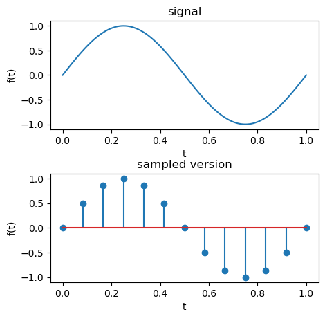
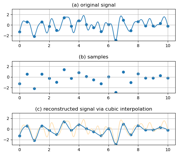
This is effectively illustrated in a second example below. The top curve is an analogue signal and the dots represent the sampling points. The sampled time series is shown in the middle, and the reconstructed signal, obtained by joining the dots in (b) is given at the bottom. Notice how much information is lost.

import numpy as np
import matplotlib.pyplot as plt
from scipy.interpolate import pchip_interpolate

t = np.linspace(0,10,1261)
F = np.sqrt(np.linspace(0.04,5,10))
A = np.array([0.5, 0.64, -0.95, -0.34, 0.2, 0.15, 0.1, 0.28, -0.31, 0.18])
w = A * np.arange(1,11) * 19.12

# construct original signal
x = t * 0
for ii in range(len(F)):
    x = x + A[ii] * np.sin(2*np.pi*F[ii]*t + w[ii])
    
# sample
t_sample = t[np.arange(0, 1261, 63)]
x_sample = x[np.arange(0, 1261, 63)]

# reconstructed signal
x_reconstruct = pchip_interpolate(t_sample, x_sample, t)

fig = plt.figure(figsize=[7,6], dpi=100)
gs = fig.add_gridspec(8, 1)
plt.subplot(gs[0:2, :])
plt.scatter(t_sample, x_sample)
plt.plot(t, x)
plt.grid()
plt.ylim(-3,3)
plt.title('(a) original signal')

plt.subplot(gs[3:5, :])
plt.scatter(t_sample, x_sample)
plt.grid()
plt.ylim(-3,3)
plt.title('(b) samples')

plt.subplot(gs[6:, :])
plt.plot(t, x, color="navajowhite", label='original')
plt.plot(t, x_reconstruct, label='reconstructed')
plt.scatter(t_sample, x_sample)
plt.grid()
plt.ylim(-3,3)
#plt.legend(loc='upper left')
plt.title('(c) reconstructed signal via cubic interpolation')

plt.show()

In order to retain all of the information that is in the initial signal, it is necessary to sample so that you have at least two samples per cycle for the highest frequency that is present in your data. If you sample a sinusoid with frequency of 50 Hz then your sampling interval must be less than or equal to 0.01 seconds - in other words, a 50 Hz sinusoid must be sampled at least 100 times per second. If you sample a complicated signal made up of many frequencies, say from 50 hz out to 300 hz (like a typical seismic signal), you must sample this signal with at least 600 samples per second in order to recover the signal accurately.

If you have a fixed sampling interval (for example, you only took measurements every 5 meters along a line), what is the highest signal frequency you could recover from the data? The question is so important that there is a name for the highest frequency sinusoid that can be recovered: it is called the Nyquist frequency and its formula is

\[ f_N = \frac{1}{2\Delta t} \]

where \(\Delta t\) is the sampling interval. If the frequency of a signal in your data exceeds the Nyquist frequency (or equivalently if your sample interval is too large and you have fewer than two samples per cycle) then you will in fact recover a sinusoid that has a lower frequency than the real signal. The phenomenon is called “aliasing”. The next figure illustrates why it happens:

import numpy as np
import matplotlib.pyplot as plt

def aliasing(f_input, f_Nyquist):
    '''
    Determine aliased frequency and the sign of the aliased signal
    
    Input Parameters:
    ----------------
    
    f_input:       original frequency
    f_Nyquist:     Nyquist frequency of the samples
    
    Return:
    ------
    
    f_output:      aliased frequency
    sign:          sign of the aliased signal
    
    '''
    f_aliased = np.abs(np.mod(f_original + f_Nyquist, 2*f_Nyquist) - f_Nyquist)
    sign = np.sign(np.mod(f_original + f_Nyquist, 2*f_Nyquist) - f_Nyquist)
    return f_aliased, sign

# time
t = np.linspace(0,4.25,201)

# original sinusoidal
f_original = 1.25       # Hz
x = np.sin(2*np.pi*f_original * t)

# Nyquist frequency of the samples
fN = 0.5                # Hz
# sample points
t_sample = np.arange(0,4.25, 1/(2*fN))
x_sample = np.sin(2*np.pi*f_original * t_sample)

# aliased sinusoidal
f_aliased, sign = aliasing(f_original, fN)
xa = sign * np.sin(2*np.pi*f_aliased * t)

# input freq
f_input = np.arange(0,2.6,0.1)
f_output = np.abs(np.mod(f_input + fN, 2*fN) - fN)

fig = plt.figure(figsize=[7,5], dpi=100)
gs = fig.add_gridspec(7,1)
plt.subplot(gs[0:3, :])
plt.plot(t,x,'-',color='k',label='original sinusoidal: f=%.2f Hz' % f_original)
plt.plot(t_sample,x_sample,'o',color='k',label='samples: fN = %.2f Hz' % fN)
plt.plot(t,xa,'--',color='coral',label='aliased sinusoidal: f=%.2f Hz' % f_aliased)
plt.legend()
plt.grid()
plt.title('original signal and aliased signal')

plt.subplot(gs[4:, :])
plt.plot(f_input,f_output)
plt.vlines(fN*np.arange(1,5),0,0.6,linestyles='dashed',color='black')
plt.scatter(f_original,f_aliased,marker='+',s=200,color='r')
for ii in range(1,5):
    plt.text(fN*ii-0.06,0.65,"$%d\ f_N$" % ii,fontsize=12)
plt.xlabel('input frequency (Hz)')
plt.ylabel('output frequency (Hz)')
plt.xlim(0,2.5)
plt.ylim(0,0.8)
plt.xticks(np.arange(0,2.6,0.25))
plt.yticks(np.arange(0,0.8,0.25))
plt.grid()
plt.title('output (aliased) frequency as a function of input frequency')
plt.show()

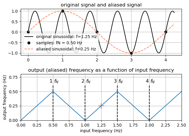
Aliasing can have disastrous consequences when interpreting geophysical data, and it should be guarded against whenever possible. Proper observation begins by knowing the highest frequency (or wavenumber for spatial signals) in the signal and choosing a sampling interval accordingly. This is generally possible in time-recordings, but it is more difficult in the spatial domain because earth structure near the surface can give rise to high frequency (or more correctly, high wavenumber) signals.

Signals depicted in time or frequency

Here is one more example of aliasing. This figure introduces a new kind of graph - the spectrum. Normal plots of data show signal strength versus time or position. A spectrum plots the signal strength versus frequency. The x-axis has units of Hertz (cycles per second). The spectrum of a signal that is a combination of two sinusoids will look like two spikes (as shown below).

f = lambda t: 5*np.cos(2*np.pi*12.5*t) + 2*np.sin(2*np.pi*75*t)
t2ms = np.linspace(0,1,int(1/0.002)+1)
t4ms = np.linspace(0,1,int(1/0.004)+1)
t8ms = np.linspace(0,1,int(1/0.008)+1)

x2ms = f(t2ms)
x4ms = f(t4ms)
x8ms = f(t8ms)

F2ms = np.fft.rfft(x2ms)
F4ms = np.fft.rfft(x4ms)
F8ms = np.fft.rfft(x8ms)

# compute spectral density
p = lambda z: (abs(np.real(z))/(np.size(z)/2),abs(np.imag(z))/(np.size(z)/2))

p2ms = p(F2ms)
p4ms = p(F4ms)
p8ms = p(F8ms)

fig = plt.figure(figsize=[8,6], dpi=100)
gs = fig.add_gridspec(8, 9)
plt.subplot(gs[0:2, 0:5])
plt.plot(t2ms,x2ms)
plt.xlim(0,1)
plt.ylim(-7,7)
plt.xlabel('t (s)')
plt.title('sampling rate = 2 ms')

plt.subplot(gs[0:2, 6:])
plt.plot(abs(F2ms)/(np.size(x2ms)/2))
plt.xlim(0,250)
plt.ylim(0,4)
plt.xticks(np.arange(0,300,50))
plt.xlabel('frequency (Hz)')
plt.ylabel('amplitude spectra')

plt.subplot(gs[3:5, 0:5])
plt.plot(t4ms,x4ms)
plt.xlim(0,1)
plt.ylim(-7,7)
plt.xlabel('t (s)')
plt.title('sampling rate = 4 ms')

plt.subplot(gs[3:5, 6:])
plt.plot(abs(F4ms)/(np.size(x4ms)/2))
plt.xlim(0,250)
plt.ylim(0,4)
plt.xticks(np.arange(0,300,50))
plt.xlabel('frequency (Hz)')
plt.ylabel('amplitude spectra')

plt.subplot(gs[6:, 0:5])
plt.plot(t8ms,x8ms)
plt.xlim(0,1)
plt.ylim(-7,7)
plt.xlabel('t (s)')
plt.title('sampling rate = 8 ms')

plt.subplot(gs[6:, 6:])
plt.plot(abs(F8ms)/(np.size(x8ms)/2))
plt.xlim(0,250)
plt.ylim(0,4)
plt.xticks(np.arange(0,300,50))
plt.xlabel('frequency (Hz)')
plt.ylabel('amplitude spectra')

plt.show()

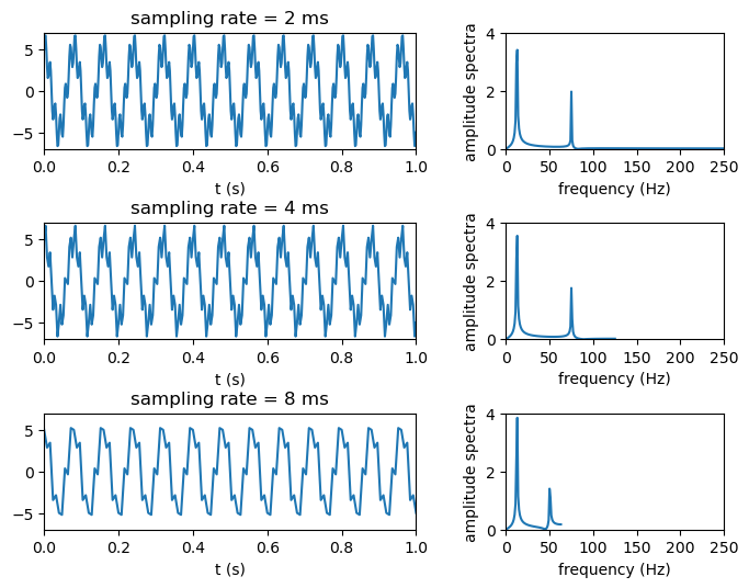
Figure: A time series syntesized from two sinusoids at 12.5 and 75 Hz at 2-ms sampling rate remains unchanged when resampled at 4 ms. However, at 8 ms, its high frequency component shifts from 75 to 50 Hz, while its low-frequency component remains the same.

Signal processing

The signal is not clear in the plot when the noise level is comparable or larger then the signal. A general method to make the wanted signal clearer is to use signal processing. One common method to improve the signal-to-noise ratio is to repeat readings and take their average: The signal parts of each reading add, whereas the noise, usually being random, tends to cancel. This is called stacking.

In the example below, the same signal from the previous SNR example is generated 100 times with different random noises. Then, the 100 signals are summed together. Notice how much the signal-to-noise ratio improves.

Previous SNR Example:

t = np.linspace(0,10,201)
x_noise = 10 * np.random.normal(0,1,size=np.shape(t))

# noise level
P_noise = np.var(x_noise)
P_noise_dB = 10 * np.log10(P_noise)

# now add a sinusoidal wave with an amplitude of 5 (smaller than the noise)
x_signal =  5 * np.sin(2*np.pi/2*t)

# signal level
P_signal = np.var(x_signal)
P_signal_dB = 10 * np.log10(P_signal)

# SNR
snr = P_signal / P_noise
snr_dB = P_signal_dB - P_noise_dB

# the sum of signal and noise
x_all = x_signal + x_noise

plt.figure(figsize=[6,3], dpi=100)
plt.plot(t,x_all)
plt.grid()
plt.xlabel('t')
plt.ylabel('x(t)')
plt.title('SNR = %.2f (%.2f dB)' % (snr, snr_dB))
plt.show()

print('Signal : P = %.2f (%.2f dB)' % (P_signal, P_signal_dB))
print('Noise  : P = %.2f (%.2f dB)' % (P_noise, P_noise_dB))
print('SNR    :     %.2f (%.2f dB)' % (snr, snr_dB))

Signal : P = 12.44 (10.95 dB)
Noise  : P = 86.43 (19.37 dB)
SNR    :     0.14 (-8.42 dB)

Stacking example:

# we can reduce the noise level by perform stacking
t = np.linspace(0,10,201)
x_individuals = np.zeros((100, np.size(t)))
x_noises = np.zeros((100, np.size(t)))
x_signals = np.zeros((100, np.size(t)))
for ii in range(100):
    x_noises[ii,:] = 10 * np.random.normal(0,1,size=np.shape(t))
    x_signals[ii,:] =  5 * np.sin(2*np.pi/2*t)
    
x_individuals = x_noises + x_signals
x_all100 = np.sum(x_individuals, axis=0)

# in this example, we know that the total signal is the sum of individual signals
x_signal100 = 100 * (5 * np.sin(2*np.pi/2*t))

# thus, the noise is the total time-series data subtracted by the signal
x_noise100 = x_all100 - x_signal100

# noise level
P_noise100 = np.var(x_noise100)
P_noise100_dB = 10 * np.log10(P_noise100)

# signal level
P_signal100 = np.var(x_signal100)
P_signal100_dB = 10 * np.log10(P_signal100)

# SNR
snr100 = P_signal100 / P_noise100
snr100_dB = P_signal100_dB - P_noise100_dB

####################################################################
# stats for the individual trace
trace_no =23

# noise level 
P_noise_individual = np.var(x_noises[trace_no,:])
P_noise_individual_dB = 10 * np.log10(P_noise_individual)

# signal level
P_signal_individual = np.var(x_signals[trace_no,:])
P_signal_individual_dB = 10 * np.log10(P_signal_individual)

# SNR
snr_individual = P_signal_individual / P_noise_individual
snr_individual_dB = P_signal_individual_dB - P_noise_individual_dB

plt.figure(figsize=[6,5], dpi=100)
plt.subplot(2,1,1)
plt.plot(t,x_individuals[23,:])
plt.tick_params(
    axis='x',          # changes apply to the x-axis
    which='both',      # both major and minor ticks are affected
    bottom=False,      # ticks along the bottom edge are off
    top=False,         # ticks along the top edge are off
    labelbottom=False) # labels along the bottom edge are off
plt.ylabel('x(t)')
plt.grid()
plt.title('An example of individual time-series: SNR = %.2f (%.2f dB)' % (snr_individual, snr_individual_dB))

plt.subplot(2,1,2)
plt.plot(t,x_all100)
plt.grid()
plt.xlabel('t')
plt.ylabel('x(t)')
plt.title('Stacked times-series: SNR = %.2f (%.2f dB)' % (snr100, snr100_dB))
plt.show()

print('Signal : P = %.2f (%.2f dB)' % (P_signal100, P_signal100_dB))
print('Noise  : P = %.2f (%.2f dB)' % (P_noise100, P_noise100_dB))
print('SNR    :     %.2f (%.2f dB)' % (snr100, snr100_dB))

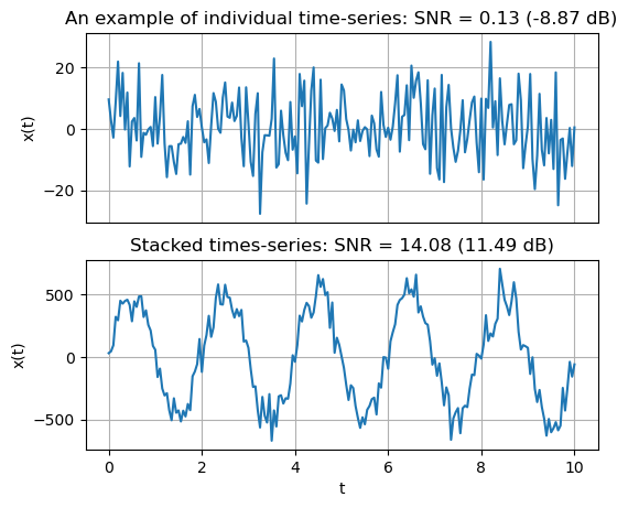
Signal : P = 124378.11 (50.95 dB)
Noise  : P = 8832.30 (39.46 dB)
SNR    :     14.08 (11.49 dB)

Another way to remove the noise is applying moving-average. The moving-average acts as a low-pass filter allowing the low-frequency sinusoidalsk to pass while filtering out the high-frequency ones. note that the random noise is a combination of sinusoidal waves with a wide rage of frequencies including the very high-frequency ones.

# the same example of the noise and the signal
# the sample rate is 20 Hz
t = np.linspace(0,10,201)
x_noise = 10 * np.random.normal(0,1,size=np.shape(t))

# now add a sinusoidal wave with an amplitude of 5 (smaller than the noise)
x_signal =  5 * np.sin(2*np.pi/2*t)

# the sum of signal and noise
x_all = x_signal + x_noise

# running average of 10 samples (~1 s or 1 Hz)
length_average = 20

# A trick to do moving average without using loops!
# It uses the concept of convolution which is useful for signal (image) 
# processing. You are not suppose to know how it works yet. You can just use 
# a couple lines of code below. All you need to change is the length of the 
# moving average.
v = np.ones(length_average) / length_average
x_all_moving = np.convolve(x_all, v, 'same')

plt.figure(figsize=[6,5], dpi=100)
plt.subplot(2,1,1)
plt.plot(t, x_signal)
plt.grid()
plt.ylim(-30,30)
plt.ylabel('x(t)')
plt.title('clean signal')

plt.subplot(2,1,2)
plt.plot(t, x_all, color='orange', linewidth=1, label="original data")
plt.plot(t, x_all_moving, '--b', linewidth=2, label="moving average: length = %d" % length_average)
plt.grid()
plt.xlabel('t')
plt.ylabel('x(t)')
plt.ylim(-30,30)
plt.legend()
plt.show()

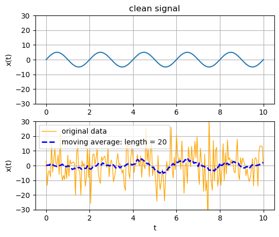
The appropriage running length of the moving average depends on the target frequency of the signal we want to have. The rule of thumb is the frequency above the \(1 / (n \Delta t)\) is going to be filtered by the moving avarage when \(n\) is the running length, and \(\Delta t\) is the sampling interval.

Question 2 You are in charge of surveying a 10x10 km area for finding a really strong 10x10 m target anomaly at a depth of 10-100 m. How will you decide on the sampling of your measurements in space and time to optimize the use of your resources (i.e. time and money)?

Answer

---

Part III: Magnetometer Survey near Princeton

The exercise will be a magnetometer survey along the towpath that follows the Delaware-Raritan canal (see map below). Somewhere north of the Blackwells Mills road parking lot is a target beneath the footpath. The goal of this survey is to find it, delineate its size, and to subsequently interpret the nature of the anomalous rock formation. The survey will be performed by teams of 2 people, each using a magnetometer. A key challenge of the survey will be designing the measurement line (i.e. how often to measure, where, etc), and in keeping careful records of locations and values of individual measurements. The latter part is essential for successful inverse modeling of the observed data.

Practical considerations:

The Geophysics Field Day will run from 9 AM - 2 PM. We will travel about 25 minutes from campus to the field site on the Delaware-Raritan Canal along the border of Hillsborough and Franklin Townships.

• You will work outside for a couple of hours. Please dress accordingly! Wear comfortable clothes and sturdy shoes.

• You will work through the normal lunch hour – bring a sandwich! Bring a water bottle or whatever else you need to drink for the day.

• Do NOT wear belts, jewelry or bring any other metallic objects/electronics except a smartphone/laptop.

Equipment:

For each participant:

• Bring your laptop, something to write with and a pad of paper or notebook. We’ll provide clipboards.

• On your laptop, install Anaconda to run Jupyter notebooks without internet access: Installation Link

• Make sure you have the Gauges app loaded onto your smart phone. See links below - upgrade to paid version so that you can record the data.

  • For iphone: Installation Link

  • For android phones: Installation Link

• In the Gauges app settings, turn OFF the CSV Options that asks to include metadata “Sep=”. This makes your data easier to load in Pandas.

• Make sure you have a Stopwatch app that can record time intervals.

For teams:

• Select your Smartphone; newer ones tend to have better hardware.

• Select your Laptop; you will need to sync data from your Smartphone so compatibility helps (e.g. Mac with iPhone).

• Your Casing:

  • Wooden Ice Hockey Stick

  • Wooden Toy truck

• 2 Tape measures (unless markers are already in place)

• 24 Wooden Stakes or Flags (unless markers are already in place)

Instrument Assembly

• Operators of magnetometers should leave anything strongly magnetic in the van (e.g. belts, earrings).

• Magnetometer crew needs to have 2 people:

  1. One holds the magnetometer

  2. Another follows atleast 5 meters behind with the laptop.

• Assemble your magnetometer by removing any smartphone case and attaching the phone to the casing with zipties.

Survey Logs

After your magnetometer has been assembled, it is a good time to take a pause to admire the beautiful scenery! Delaware and Raritan Canal first opened in 1834 and provided a direct transportation link between the cities of Philadelphia and New York City. For nearly a century, the D&R Canal was one of America’s busiest navigation canals. What was once a thoroughfare for mule-powered canal boats, steam-powered vessels and pleasure boats of all kinds, is today central New Jersey’s most popular recreational corridor offering a serene and surprising respite from the commotion of major cities and expressways.

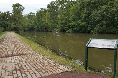
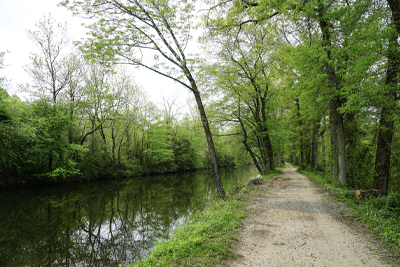
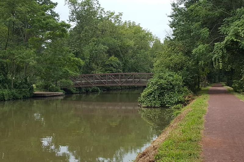
Figure: Snapshots of the Delaware and Raritan Canal. Source: New Jersey State Park Service

TO DO

Question 3.1: Write down all relevant details of this survey such as the time, team members, date, address and GPS coordinates where your survey began from the Gauges app.

Answer

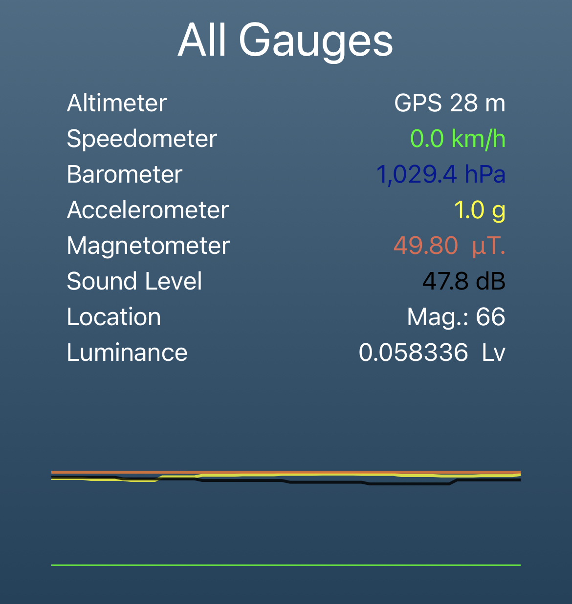
Question 3.2: List typical values of all gauges reported by the Gauges app (e.g. altimeter, barometer) while your instrument is standing still. These should be at the bottom of the app window and look like the snapshot below:

Answer

Question 3.3: Describe in 1 or 2 lines each what property of the Earth or your surrounding each gauge on the Gauges app measures.

Answer

Question 3.4: 1) Take any good photo for memory with your camera and 2) Make a map-view sketch of the target and survey region (if you discover one). Upload a scanned copy with this assignment and geotag both by reporting their GPS coordinates below. Note: You can wait till you have explored the survey area before sitting down to make a sketch!

Answer

Phase I: Noise Calibration

• Upon arrival at the field site carry your magnetometer onto the towpath, and walk with it around 50 m North of the entry gate.

• Mark the position where the survey will begin with GPS, reporting in in Question 3.1 above. An alternative strategy is sometimes to find a good landmark that may be tagged to a Google Earth image at a later time.

• Change the settings on the Gauges app to have an update interval of 100 ms (i.e. 10 samples every second). This is our default sampling interval for our time domain signal (\(\Delta t\)). We might need to adjust this later based on your survey design!

• Press the record button on the Gauges app, walk along the tow path slowly with your magnetometer (1 step every second) for a few meters in front of you (longer the better).

• Stop recording, open the file folder on the Gauges app and transfer the file to your computer. Rename the file as calibration-CASING-PUID.csv where CASING is the casing is either truck or hockey.

• Redo this recording for both types of casing and perform the following calculations. Make sure to walk at a similar pace when doing both types, in order to facilitate comparisons.

TO DO

Question 4: 1) Report the Nyquist frequency of your time domain signal. 2) We will treat the results from this phase where are simply calibrating our magnetometer at the beginning of the survey as representing the noise level. Report the noise level of your two types of casing for magnetometers in dB. Which casing is noisier? Speculate on the possible reasons.

Answer

Phase II: Prior Information

When geophysicists head out to the field, they are never completely in the dark about the target! There are often prior observations or historical knowledge that inform the survey design such as the choice of instruments. Two major sources of information are available for this area of Central New Jersey.

Typical Rocks and Geological Maps

Princeton and adjoining areas are part of the Piedmont physiographic province and the Newark basin. The rocks of the Piedmont are of Late Triassic and Early Jurassic age (230 to 190 Ma). They rest on a large, elongate crustal block that dropped downward in the initial stages of the opening of the Atlantic Ocean, one of a series of such blocks in eastern North America. These downdropped blocks formed valleys known as rift basins. Sediment eroded from adjacent uplands was deposited along rivers and in lakes within the basins. These sediments became compacted and cemented to form conglomerate, sandstone, siltstone, and shale.

In the course of rifting, the rock layers of the Piedmont became tilted northwestward, gently folded, and cut by several major faults. The Newark basin is perhaps the most extensively studied of the early Mesozoic basins of eastern North America that formed during the breakup of Pangea. The basin is around 190 km long and a maximum of 50 km wide. Volcanic activity was also associated with the rifting, as indicated by the basalt and diabase interlayered with sandstone and shale. Diabase is a rock formed by the cooling of magma at some depth in the crust; basalt is formed by cooling of an identical magma that has been extruded onto the surface as lava.

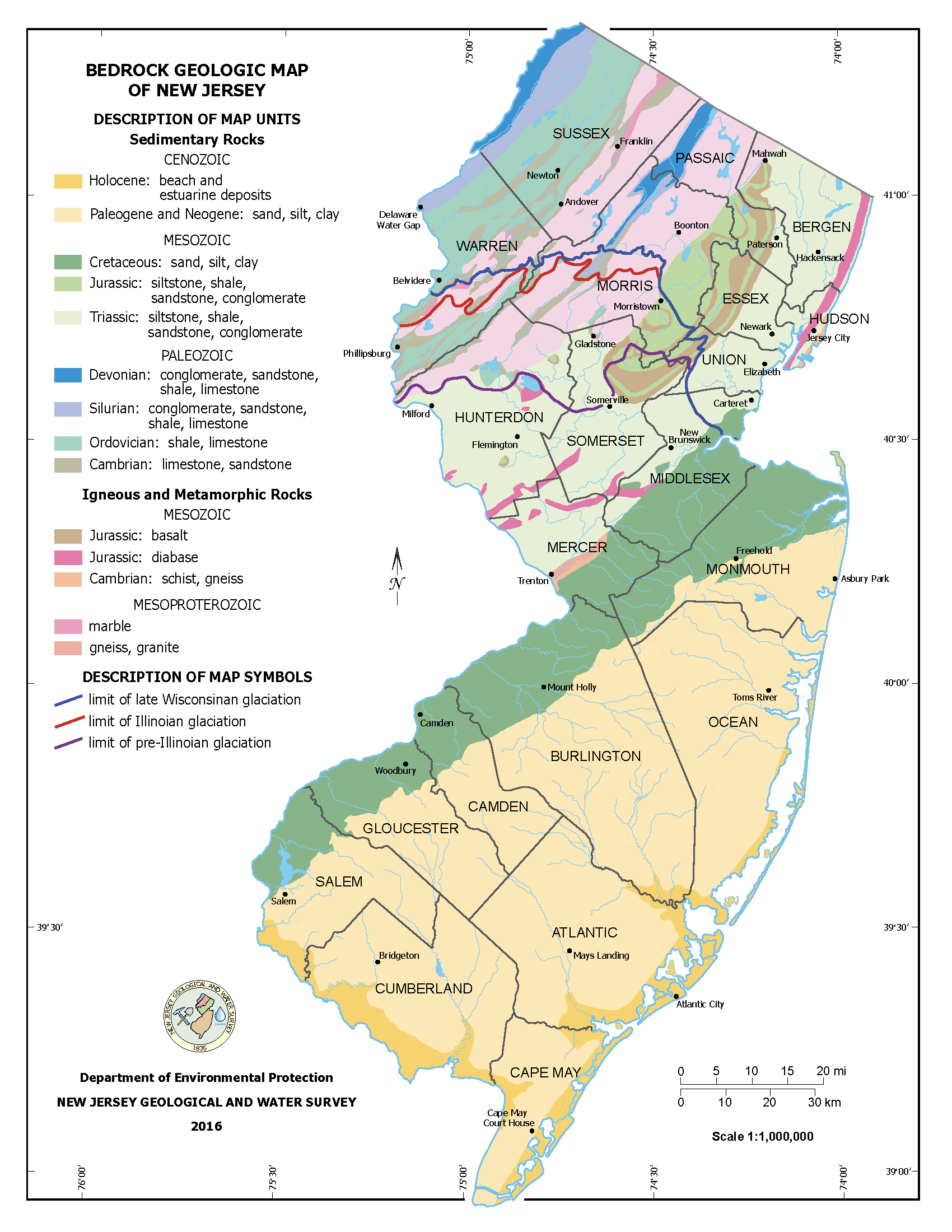
Magnetic Properties of Rocks

Before considering magnetic anomalies as a way to detect a target, we consider the topic of magnetic susceptibility and to review several other considerations relevant to computation of magnetic intensities. Recall that we elected to use the cgs system of units in this chapter. Although susceptibility is dimensionless, values normally are expressed as cgs or emu (electromagnetic units) to call attention to the fact that cgs units are in use rather than SI units. The susceptibility values given here can be converted to SI units by multiplying by 4\(\pi\). Although several familiar minerals have high susceptibilities (magnetite, ilmenite, and pyrrhotite), magnetite is by far the most common. Rock susceptibility almost always is directly related to the percentage of magnetite present. The true susceptibility of magnetite varies from 0.1 to 1.0 emu depending on grain size, shape, and impurities. Average susceptibility as quoted in several sources ranges from 0.2 to 0. 5 emu, so we will adopt a value of k = 0.35 emu for our computation. Representative values for a selection of common rocks and minerals are presented in Telford, Geldart, and Sheriff (1990, 74). For our discussions of anomaly interpretation, it is enough to concentrate on average susceptibilities for common rock groups.

Rock type	Susceptibility (emu=SI/4\(\pi\))
Sedimentary rocks	0.00005 emu
Metamorphic rocks	0.0003 emu
Granites and rhyolites	0.0005 emu
Gabbros and basalts	0.006 emu
Ultrabasic rocks	0.012 emu

TO DO

Question 5: Based on the two types of prior information outlined above, what are the major types and ages of rocks in our field survey area? Based on the magnetic susceptibilities, what kind of common rock type as targets will create strong magnetic anomalies?

Answer

Phase III: Prospecting

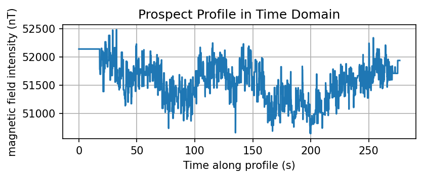
Start walking at a slow pace along the towpath northwards, recording your measurements on the Gauges app. You are welcome to go as far as you want from the starting point for this first pass of prospecting for the target. However, a distance of 500 m should be appropriate to start. At the end of this first pass, download the Gauges data to your computer and name the file as Gauges_Prospecting-PUID.csv, which should be similar to Magnetic_reading_example.csv.

TO DO

Question 6: Make a profile of the magnetic field intensity in nanoTeslas (nT) as a function of time elapsed along your prospecting profile. Do you see any signal that could correspond to a target of interest? If yes, note down the range in time where it is detected. What is the shape of this signal and how large is the signal amplitude in nT? You may modify the code provided below.

Answer

Modify the code below

##############   USER DEFINED    ###################
gauges_file = 'Files/Magnetic_reading_example.csv'
####################################################

import numpy as np
import pandas as pd
import matplotlib.pyplot as plt
from scipy.interpolate import interp1d
from scipy.signal import detrend
from pathlib import Path

data_forward = pd.read_csv(gauges_file)
data_forward.columns

Index(['Date', 'Speed', 'Altitude', 'Pressure', 'X', 'Y', 'Z', 'G', 'Latitude',
       'Longitude', 'Heading', 'Magnetic Field', 'Sound Level', 'Luminance',
       'Heart Rate'],
      dtype='object')

data_forward['Date'] = pd.to_datetime(data_forward['Date'])
data_forward['Difference'] = data_forward['Date']-data_forward['Date'][0]
Time_seconds = []
for val in data_forward['Difference']: Time_seconds.append(val.total_seconds())
data_forward['Time_seconds'] = Time_seconds
data_forward['Magnetic_Field_nT'] = data_forward['Magnetic Field']*1000

plt.figure(figsize=[6,2], dpi=150)
plt.plot(data_forward['Time_seconds'],data_forward['Magnetic_Field_nT'])
plt.grid()
plt.xlabel('Time along profile (s)')
plt.ylabel('magnetic field intensity (nT)')
plt.title('Prospect Profile in Time Domain')
plt.show()

Phase IV: Data Acquistion

Note that the X-axis of the profile is in terms of time elapsed, while you are interested in the spatial extent (e.g. size, depth) of a target. A conversion to distance along the profile is needed for each reading. GPS is widely used for finding (approximate) locations, but the uncertainties of these values can be large depending on various factors such as the number of satellites used for triangulation. We will go the old-fashioned way instead!

Use tape measure and flags (or wooden stakes) to mark locations every 20 meters where measurements will be made. The profile that you plan should ideally be centered on the target that you may have detected while prospecting. The footpath is made of gravel and people might be running or biking, so marking along the grass is a decent strategy.

IMPORTANT once you find the anomaly, make sure you establish its entire shape by making the measurements on both direction away from the anomaly. You should find that the field will eventually return to the value similar to that at the start of the survey.

In Microsoft excel, create a CSV file called Stakes_Run_1-PUID.csv, which should be similar to Stakes_example.csv. Download the Gauges data to your computer and name the file as Gauges_Run_1-PUID.csv, which should be similar to Magnetic_reading_example.csv. We will use the helper function below to convert from time to distance domain along the profile. Since we walked at an uneven pace (because we are human after all!), we took readings unevenly spaced in distance even though we adopted a uniform sampling interval in time! We therefore find the nearest readings through interpolation to create a profile evenly spaced in distance. A uniform sampling interval makes signal processing way easier, especially for stacking or a running moving average!

DO NOT modify the code below

def read_gauges_data(gauges_file):
    '''
    Reads CSV file from Gauges app and adds some field
     
    Input Parameters:
    ----------------
    
    gauges_file:         CSV file output from Gauges
    
    Return:
    ------
    
    df:                  Pandas Dataframe with Time_seconds and Magnetic_Field_nT columns
    '''

    data_forward = pd.read_csv(gauges_file)
    data_forward['Date'] = pd.to_datetime(data_forward['Date'])
    data_forward['Difference'] = data_forward['Date']-data_forward['Date'][0]
    Time_seconds = []
    for val in data_forward['Difference']: Time_seconds.append(val.total_seconds())
    data_forward['Time_seconds'] = Time_seconds
    data_forward['Magnetic_Field_nT'] = data_forward['Magnetic Field']*1000
    return data_forward

def get_uniform_profile(df_reading, df_stake, dx):
    '''
    Calculate the magnetic field along a profile with a uniform spacing
    
    Input Parameters:
    ----------------
    
    df_reading:          Pandas Dataframe containing reading
    df_stake:          Pandas Dataframe containing stakes
    dx:                distance interval spacing for the output
    
    Return:
    ------
    
    x_uniform:         locations along the profile
    B_uniform:         magnetic field along the profile
    
    '''

    #t_reading:         reading time of the observation
    #B_reading:         magnetic field at t_reading
    t_reading = np.array(df_reading['Time_seconds'])
    B_reading = np.array(df_reading['Magnetic_Field_nT'])
    
    #t_stakes:          time when the instrument is at a stake
    #x_stakes:          location of the stakes along the profile
    t_stakes = np.array(df_stake['Time_seconds'])
    x_stakes = np.array(df_stake['Location_m'])

    # convert to time from reading to distance assuming the constant speed between 2 stakes
    t_reading_to_x_reading = interp1d(t_stakes, x_stakes, 'linear', fill_value="extrapolate")
    x_reading = t_reading_to_x_reading(t_reading)
    
    # resampling for uniform sampling interval
    x_uniform = np.arange(x_stakes[0], x_stakes[-1], dx)
    
    # interpolate the magnetic field from the reading locations to the uniform intervals
    B_reading_to_B_uniform = interp1d(x_reading, B_reading, 'nearest')
    B_uniform = B_reading_to_B_uniform(x_uniform)
    
    return x_uniform, B_uniform

TO DO

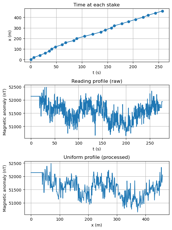
Question 7: Make a profile of the magnetic field intensity in nanoTeslas (nT) as a function of location in meters along your prospecting profile. What is the Nyquist frequency of the time series evenly sampled in location? How broad is the anomaly in meters? Adjust your sampling rate (i.e. walking faster or slower) for future runs based on the detectability with your current parameters.

Answer

Modify the code below

##############   USER DEFINED    ###################
stake_fname = 'Files/Stakes_example.csv'
reading_fname = 'Files/Magnetic_reading_example.csv'
sampling_interval = 1 # sampling interval in m
####################################################

df_reading = read_gauges_data(reading_fname)
df_stake = pd.read_csv(stake_fname)

# resampling for uniform sampling interval
x_uniform, B_uniform = get_uniform_profile(df_reading, df_stake, sampling_interval)

plt.figure(figsize=[6,8], dpi=100)
plt.subplot(3,1,1)
plt.plot(df_stake.Time_seconds,df_stake.Location_m, '-o')
plt.xlabel('t (s)')
plt.ylabel('x (m)')
plt.grid()
plt.title('Time at each stake')

plt.subplot(3,1,2)
plt.plot(df_reading.Time_seconds, df_reading.Magnetic_Field_nT)
plt.xlabel('t (s)')
plt.ylabel('Magnetic anomaly (nT)')
plt.grid()
plt.title('Reading profile (raw)')

plt.subplot(3,1,3)
plt.plot(x_uniform, B_uniform)
plt.grid()
plt.xlabel('x (m)')
plt.ylabel('Magnetic anomaly (nT)')
plt.title('Uniform profile (processed)')

plt.tight_layout()
plt.show()

Phase V: Signal Processing

In order to accentuate the signal from the noise, some processing is required on the fly. Try out the options below.

TO DO

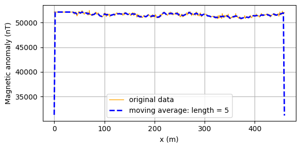
Question 8.1: Based on experimentation with a range of values with the code below and guideline discussed in the text above, what length of the running window is appropriate for your survey?

Answer

Question 8.2: Calculate the signal power of the target in dB for a single profile, moving average and stacking of multiple runs. What is the SNR for each case if noise dB is the value from Question 4.

Answer

Moving average

##############   USER DEFINED    ###################
length_average = 5 # number of samples to average in a running window
#####################################################
v = np.ones(length_average) / length_average
B_uniform_moving = np.convolve(B_uniform, v, 'same')

plt.figure(figsize=[6,3], dpi=100)
plt.plot(x_uniform, B_uniform, color='orange', linewidth=1, label="original data")
plt.plot(x_uniform, B_uniform_moving, '--b', linewidth=2, label="moving average: length = %d" % length_average)
plt.grid()
plt.xlabel('x (m)')
plt.ylabel('Magnetic anomaly (nT)')
plt.legend()

plt.tight_layout()
plt.show()

Stacking

##############   USER DEFINED    ###################
# list of files to interpolate and stack
files_to_stack = ['Files/Magnetic_reading_example.csv'] 
stakes_fnames = ['Files/Stakes_example.csv']
reading_fnames = ['Files/Magnetic_reading_example.csv']
sampling_interval = 1 # sampling interval in m
####################################################

num_profiles=len(files_to_stack)
num_stacks=len(stakes_fnames)
assert(num_profiles==num_stacks)

df_reading = read_gauges_data(reading_fnames[0])
df_stake = pd.read_csv(stakes_fnames[0])

# resampling for uniform sampling interval
x1, B1 = get_uniform_profile(df_reading, df_stake, sampling_interval)

x_all = np.empty((num_profiles, len(x1)))
B_all = np.empty((num_profiles, len(B1)))

x_all[0] = x1
B_all[0] = B1

if num_profiles>1:
    for ii,reading in enumerate(reading_fnames):
        df_reading = read_gauges_data(reading)
        df_stake = pd.read_csv(stakes_fnames[ii])        
        x_all[ii], B_all[ii] = get_uniform_profile(df_reading, df_stake, sampling_interval)
    
# stack all measurements together
B_sum = np.sum(B_all, axis=0)

plt.figure(figsize=[6,5], dpi=100)
plt.subplot(2,1,1)
plt.plot(x1, B1, '-')
plt.tick_params(
    axis='x',          # changes apply to the x-axis
    which='both',      # both major and minor ticks are affected
    bottom=False,      # ticks along the bottom edge are off
    top=False,         # ticks along the top edge are off
    labelbottom=False) # labels along the bottom edge are off
plt.ylabel('Magnetic anomaly (nT)')
plt.grid()
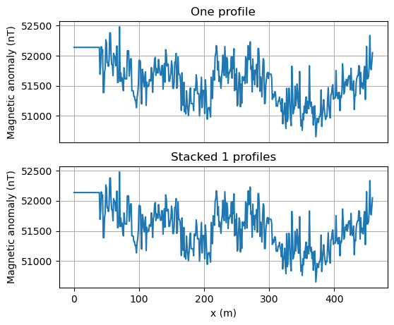
plt.title('One profile')

plt.subplot(2,1,2)
plt.plot(x1, B_sum, '-')
plt.grid()
plt.xlabel('x (m)')
plt.ylabel('Magnetic anomaly (nT)')
plt.title('Stacked %d profiles' % num_profiles)
plt.show()

Phase VI: Modeling

Several reductions or corrections are usually applied to the acquired data before the magnetic anomaly can be modeled in terms of interior structure. We will ignore both of these corrections since our survey duration and area is small enough.

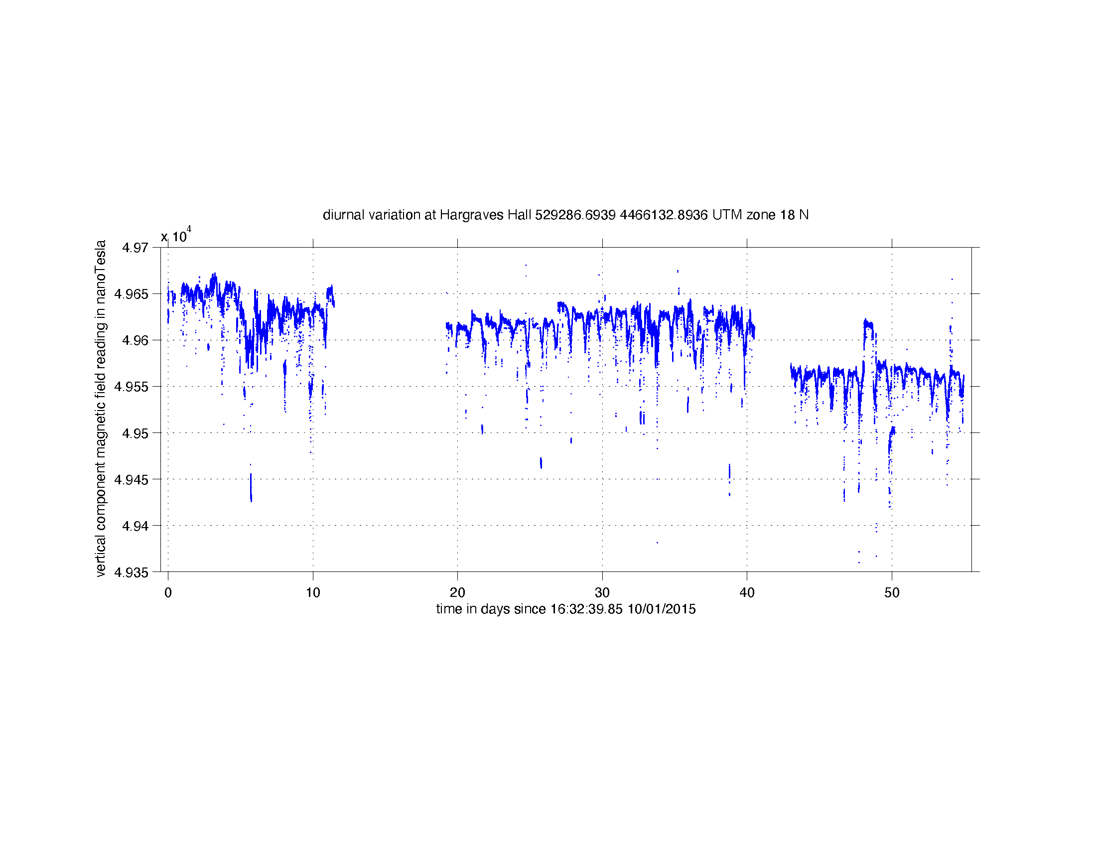
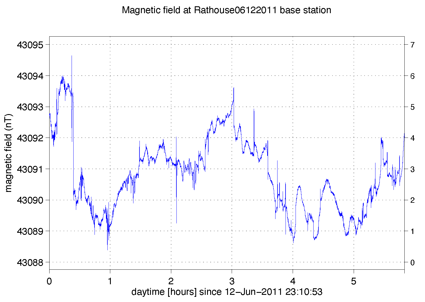
Correction 1: Diurnal variations. The strength of the Earth’s field changes over the course of a day, called diurnal variation. Variation seldom reaches as much as 100 nT over 24 hrs, but during occasional magnetic storms it can exceed 1000 nT. As the diurnal variation changes smoothly (unlike storms), it can be measured by returning periodically to the base station. Figures below show examples of diurnal variations in Princeton (Hargroves Hall) and in Cyprus. Note that there is a lot of airconditioner noise in Princeton. If the anomaly is large or the time spent recording it is short, correcting for diurnal variation may make little difference to the anomaly, but recording it provides a sanity check that the instrument is functioning correctly and that there are no magnetic storms.

Correction 2: Subtracting the global field. The magnetic field varies a lot over the Earth’s surface, being roughly twice as strong at the Earth’s magnetic poles as the equator. This variation does not matter for surveys of small areas, but is corrected during regional survey. The field subtracted is the IGRF – International Geomagnetic Reference Field, which is revised every 5 years. This field expressed as sum of spherical harmonic series (a.k.a. 2-dimensional sinusoids), and matches the actual field measured at observatories around the Earth by the fields of a series of fictitious magnets at the Earth’s centre. A decent fit is provided by a single dipole arising from the geodynamo, but progressively smaller magnets with various orientations are used to improve the match to about 1 nT on average.

Finding the depth of the body As a general rule, shallower anomalies tend to have sharper anomalies and shorter wavelengths, and this can be used to deduce the depth of the target. However, the shapes of anomalies also depend on the direction of magnetisation, and often have both positive and negative parts. We will use Peter’s half-slope method for quick calculations of anomaly depth in the field. The slope of the steepest part of the anomaly is drawn; then a line half as steep is drawn. Next, positions A and B, either side of the steepest part, are found with the slope of line 2, and their horizontal separation, S, measured. The depth, d, to the top of the body is given approximately by depth, d ~ 1.6 S. This relationship works best for dykes or sheets aligned N–S (near-symmetric anomalies), and at high latitudes.

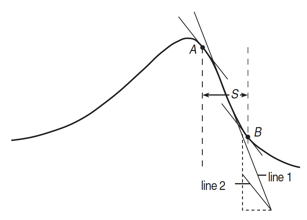
Figure: Peter’s half-slope method for estimating approximate depth of a targent.

TO DO

Question 9: Deduce the depth of your target. Speculate on its orientation based on the anomaly shape.

Answer

Phase VII: Geological interpretation

A database of geologic units and structural features in New Jersey, with lithology, age, data structure, and format written and arranged just like the other states is available from the United States Geological Survey. The information is provided in terms of shapefiles, a commonly used format for sharing geometry data. Geometry of a given feature is stored as a set of vector coordinates. We first probe the columns and types of polygons representing various types of rock formations in New Jersey. Here is an example of what the shapefile NJ_geol_poly.shp contains. Next, we choose the polygons that outline the general type of rock type called ‘Igneous, intrusive’ and plot the outline of these rock formations.

import geopandas as gpd
import json

geojson = 'Files/NJ/NJ_geol_poly_instrusive.json'

NJ_geol_poly = gpd.read_file('Files/NJ/NJ_geol_poly.shp')
print('Columns are : ',NJ_geol_poly.columns)
print('General types are : ',NJ_geol_poly.GENERALIZE.unique())

# Choose intrusive igenous formations
NJ_geol_poly[NJ_geol_poly.GENERALIZE=='Igneous, intrusive'].to_file(geojson, driver = "GeoJSON")
with open(geojson) as geofile: j_file = json.load(geofile)

Columns are :  Index(['STATE', 'ORIG_LABEL', 'SGMC_LABEL', 'UNIT_LINK', 'REF_ID',
       'GENERALIZE', 'SRC_URL', 'URL', 'geometry'],
      dtype='object')
General types are :  ['Metamorphic, sedimentary clastic' 'Sedimentary, carbonate'
 'Metamorphic, undifferentiated' 'Metamorphic, serpentinite'
 'Sedimentary, undifferentiated' 'Sedimentary, clastic'
 'Igneous, intrusive' 'Igneous, volcanic'
 'Unconsolidated, undifferentiated'
 'Metamorphic and Sedimentary, undifferentiated' 'Water'
 'Metamorphic, amphibolite' 'Metamorphic, gneiss' 'Metamorphic, carbonate']

TO DO

Question 10: Become a detective! Based on your understanding of the tectonic history of the eastern United States, figure out the type of geological feature that is the target beneath your feet?

Hints: Exploring the rock formations along the Hudson river with the choropleth map above may hold a clue. Another clue could be exposed in the roadcut on the opposite side of the canal, although it could be hidden by vegetation. Identify the rock type of the exposure to explain the history of your target anomaly.

Answer