Human Interactions
Contents
Human Interactions#
IN THE SPACE BELOW, WRITE OUT IN FULL AND THEN SIGN THE HONOR PLEDGE:
“I pledge my honor that I have not violated the honor code during this examination.”
PRINT NAME:
If a fellow student has contributed significantly to this work, please acknowledge them here:
Peer(s):
Contribution:
By uploading this assignment through Canvas, I sign off on the document below electronically.
Part I: A modified ranking of costly disasters#
The following table list some recent natural disasters, and the estimated economic losses in the affected country. The economic losses are often hard to estimate, so these are approximate values.
Year |
Event |
Country |
Economic loss |
|---|---|---|---|
2010 |
Port-au-Prince Earthquake |
Haiti |
$3 billion |
2014 |
Laudian Earthquake |
China |
$10 billion |
2005 |
Hurricane Katrina |
USA |
$150 billion |
2011 |
M9.1 Earthquake |
Japan |
$200 billion |
2012 |
Hurricane Sandy |
USA |
$150 billion |
1998 |
Hurricane Mitch |
Honduras |
$4 billion |
We will rank the severity of the disasters based on the economic losses compared with the national wealth, estimated as their gross domestic products (GDPs, Wikipedia). Here is an example on how to read a .csv file and access the data using a pandas Dataframe.
# import these packages when you read .csv file
import pandas as pd

# this one is only for making interactive plots. You do not need to import this.
import plotly.express as px
# Read a the GDP data file
data = pd.read_csv('Files/GDP_Data.csv')

# Display the content of the dataframe.
# Useful to see the column names. Pay attention to the unit of GDP.
# alternatively, you can open the .csv file
data
| Country Name | Country Code | Indicator Name | Indicator Code | 1960 | 1961 | 1962 | 1963 | 1964 | 1965 | ... | 2012 | 2013 | 2014 | 2015 | 2016 | 2017 | 2018 | 2019 | 2020 | 2021 | |
|---|---|---|---|---|---|---|---|---|---|---|---|---|---|---|---|---|---|---|---|---|---|
| 0 | Tuvalu | TUV | GDP (current US$) | NY.GDP.MKTP.CD | NaN | NaN | NaN | NaN | NaN | NaN | ... | 3.934562e+07 | 3.861749e+07 | 3.875969e+07 | 3.681166e+07 | 4.162950e+07 | 4.521766e+07 | 4.781829e+07 | 5.422315e+07 | 5.505471e+07 | 6.310096e+07 |
| 1 | Nauru | NRU | GDP (current US$) | NY.GDP.MKTP.CD | NaN | NaN | NaN | NaN | NaN | NaN | ... | 9.692720e+07 | 9.849184e+07 | 1.046544e+08 | 8.652966e+07 | 9.972339e+07 | 1.093597e+08 | 1.240214e+08 | 1.187241e+08 | 1.146266e+08 | 1.332189e+08 |
| 2 | Kiribati | KIR | GDP (current US$) | NY.GDP.MKTP.CD | NaN | NaN | NaN | NaN | NaN | NaN | ... | 1.896301e+08 | 1.845507e+08 | 1.778623e+08 | 1.702910e+08 | 1.785098e+08 | 1.881921e+08 | 1.962306e+08 | 1.779353e+08 | 1.809118e+08 | NaN |
| 3 | Marshall Islands | MHL | GDP (current US$) | NY.GDP.MKTP.CD | NaN | NaN | NaN | NaN | NaN | NaN | ... | 1.804363e+08 | 1.848404e+08 | 1.821428e+08 | 1.838143e+08 | 2.015109e+08 | 2.132041e+08 | 2.215889e+08 | 2.394622e+08 | 2.444624e+08 | 2.486656e+08 |
| 4 | Palau | PLW | GDP (current US$) | NY.GDP.MKTP.CD | NaN | NaN | NaN | NaN | NaN | NaN | ... | 2.123978e+08 | 2.211172e+08 | 2.416698e+08 | 2.804577e+08 | 2.983000e+08 | 2.853000e+08 | 2.847000e+08 | 2.742000e+08 | 2.577000e+08 | NaN |
| ... | ... | ... | ... | ... | ... | ... | ... | ... | ... | ... | ... | ... | ... | ... | ... | ... | ... | ... | ... | ... | ... |
| 261 | Sint Maarten (Dutch part) | SXM | GDP (current US$) | NY.GDP.MKTP.CD | NaN | NaN | NaN | NaN | NaN | NaN | ... | 9.858659e+08 | 1.022905e+09 | 1.245251e+09 | 1.253073e+09 | 1.263687e+09 | 1.191620e+09 | 1.185475e+09 | NaN | NaN | NaN |
| 262 | Syrian Arab Republic | SYR | GDP (current US$) | NY.GDP.MKTP.CD | 8.577044e+08 | 9.452450e+08 | 1.110566e+09 | 1.200447e+09 | 1.339494e+09 | 1.329842e+09 | ... | 4.411780e+10 | 2.255247e+10 | 2.207599e+10 | 1.762206e+10 | 1.245346e+10 | 1.634067e+10 | 2.144578e+10 | NaN | NaN | NaN |
| 263 | Turkmenistan | TKM | GDP (current US$) | NY.GDP.MKTP.CD | NaN | NaN | NaN | NaN | NaN | NaN | ... | 3.516421e+10 | 3.919754e+10 | 4.352421e+10 | 3.579971e+10 | 3.616943e+10 | 3.792629e+10 | 4.076543e+10 | 4.523143e+10 | NaN | NaN |
| 264 | Venezuela, RB | VEN | GDP (current US$) | NY.GDP.MKTP.CD | 7.779091e+09 | 8.189091e+09 | 8.946970e+09 | 9.753333e+09 | 8.099318e+09 | 8.427778e+09 | ... | 3.812860e+11 | 3.710050e+11 | 4.823590e+11 | NaN | NaN | NaN | NaN | NaN | NaN | NaN |
| 265 | British Virgin Islands | VGB | GDP (current US$) | NY.GDP.MKTP.CD | NaN | NaN | NaN | NaN | NaN | NaN | ... | NaN | NaN | NaN | NaN | NaN | NaN | NaN | NaN | NaN | NaN |
266 rows × 66 columns
# Here is an example on how to obtain Palau's GDP in 2018
Palau_2018_GDP = data[data['Country Name'] == 'Palau']['2018']
Palau_2018_GDP
4    284700000.0
Name: 2018, dtype: float64
Note that the value is not just a number but pandas series. Although you can do most arithmatic operations with pandas series, there are some certain operations that you need to use the actual number (in float data type). The example below illustrate on how to add the GDPs of two countries.
# Here is how to add two countries GDPs

# convert to float
Palau_2018_GDP = data[data['Country Name'] == 'Palau']['2018'].array[0]
Nauru_2018_GDP = data[data['Country Name'] == 'Nauru']['2018'].array[0]

sum_2018_GDP = Palau_2018_GDP + Nauru_2018_GDP

# display the sum
print("The total GDP from Palau and Nauru in 2018 is %.2g US Dollars" % sum_2018_GDP)
The total GDP from Palau and Nauru in 2018 is 4.1e+08 US Dollars
# Now we select a few nations to make a bar chart
countries = data['Country Name']

wh = ((countries == 'Honduras') |
      (countries == 'Haiti') |
      (countries == 'United States') |
      (countries == 'Japan') |
      (countries == 'China'))
data_selected = data[wh]
data_selected
| Country Name | Country Code | Indicator Name | Indicator Code | 1960 | 1961 | 1962 | 1963 | 1964 | 1965 | ... | 2012 | 2013 | 2014 | 2015 | 2016 | 2017 | 2018 | 2019 | 2020 | 2021 | |
|---|---|---|---|---|---|---|---|---|---|---|---|---|---|---|---|---|---|---|---|---|---|
| 79 | Haiti | HTI | GDP (current US$) | NY.GDP.MKTP.CD | 2.731872e+08 | 2.710660e+08 | 2.818968e+08 | 2.948834e+08 | 3.252812e+08 | 3.532518e+08 | ... | 1.370893e+10 | 1.490247e+10 | 1.513926e+10 | 1.483315e+10 | 1.398769e+10 | 1.503556e+10 | 1.645503e+10 | 1.478584e+10 | 1.450822e+10 | 2.094439e+10 |
| 97 | Honduras | HND | GDP (current US$) | NY.GDP.MKTP.CD | 3.356500e+08 | 3.562000e+08 | 3.877500e+08 | 4.102000e+08 | 4.570000e+08 | 5.086500e+08 | ... | 1.852860e+10 | 1.849971e+10 | 1.975649e+10 | 2.097977e+10 | 2.171762e+10 | 2.313623e+10 | 2.406778e+10 | 2.508998e+10 | 2.382784e+10 | 2.848867e+10 |
| 229 | Japan | JPN | GDP (current US$) | NY.GDP.MKTP.CD | 4.430734e+10 | 5.350862e+10 | 6.072302e+10 | 6.949813e+10 | 8.174901e+10 | 9.095028e+10 | ... | 6.272360e+12 | 5.212330e+12 | 4.896990e+12 | 4.444930e+12 | 5.003680e+12 | 4.930840e+12 | 5.037840e+12 | 5.123320e+12 | 5.040110e+12 | 4.937420e+12 |
| 233 | China | CHN | GDP (current US$) | NY.GDP.MKTP.CD | 5.971647e+10 | 5.005687e+10 | 4.720936e+10 | 5.070680e+10 | 5.970834e+10 | 7.043627e+10 | ... | 8.532230e+12 | 9.570410e+12 | 1.047570e+13 | 1.106160e+13 | 1.123330e+13 | 1.231040e+13 | 1.389480e+13 | 1.427990e+13 | 1.468770e+13 | 1.773410e+13 |
| 237 | United States | USA | GDP (current US$) | NY.GDP.MKTP.CD | 5.433000e+11 | 5.633000e+11 | 6.051000e+11 | 6.386000e+11 | 6.858000e+11 | 7.437000e+11 | ... | 1.625400e+13 | 1.684320e+13 | 1.755070e+13 | 1.820600e+13 | 1.869510e+13 | 1.947960e+13 | 2.052720e+13 | 2.137260e+13 | 2.089370e+13 | 2.299610e+13 |
5 rows × 66 columns
# Plot an interactive bar chart
fig = px.bar(data_selected, x='Country Name', y='2020',
             title="Countries' GDP in 2020", log_y=True)
fig.update_yaxes(title='2020 GDP')
fig.show()
The two figures below show how the total global GDP in 2020 is distributed by region and income level. Run these cells to see the pie charts showing the percentages. Hovering over each section shows you the GDP and the number of countries in each region or income level.
data = pd.read_csv('Files/GDP_region.csv')
fig = px.pie(data, values='2020',
             names='Country Name',
             title="2020 GDP by Country's Region",
             labels={'Country Name':'Region',
                     '2020':'GDP',
                     'Number of Countries':'Number of Countries'},
             hover_data=['Number of Countries'])
fig.show()
import pandas as pd
import numpy as np
import plotly.express as px
data = pd.read_csv('Files/GDP_income.csv')
fig = px.pie(data, values='2020',
             names='Country Name',
             title="2020 GDP by Country's Income Level",
             labels={'Country Name':'Income Level',
                     '2020':'GDP',
                     'Number of Countries':'Number of Countries'},
             hover_data=['Number of Countries'])
fig.show()
Run the two cells below to plot a pie chart of top 10 GDP ranking of US states.
data = pd.read_csv('Files/State_GDP_Current_Dollar.csv')
data = data[-10:]      # select top 10 states
fig = px.pie(data, values='2020',
             names='GeoName',
             title="Top 10 States GDP in 2020 (in million US current dollars)",
             labels={'GeoName':'State',
                     '2020':'GDP'}
            )
fig.show()
TO DO#
Question 1.1 Calculate the loss in each disaster as a fraction of the annual Gross Domestic Product (GDP) of the affected country in the year of the disaster. Expressed in this way, how do the disasters rank in terms of severity? Please use the values of GDP in the file Files/GDP_data.csv from the World Bank lass accessed on October 10, 2022.
Answer:
Question 1.2 For the two US disasters in the table, calculate the loss as a fraction of the annual economic output (Gross State Product or equivalent) of New York + New Jersey (for hurricane Sandy) and Louisiana (for hurricane Katrina). More than 90% of monetary losses from Katrina occurred in Louisiana, so we will restrict our analysis to this state. Please use the GDP values from Files/State_GDP_Current_Dollar.csv from the year of the disaster. Be careful about the units.
Answer:
Question 1.3 Based on your ranking of global disasters in the answers above, explore the challenges for different countries to recover from natural disasters. Substantiate your answer with some calculations on the country’s road to recovery from the disaster. For this, you can assume that on average, 5% of the GDP is used for funding recovery polices each year, and no foreign aid is provided.
(A) How many years will it take to fully recover from the economic loss in the absence of foreign aid?
(B) Comment on the utility of a system of international aid and relief (e.g. United Nations, Red Cross) in response to disasters, especially in developing countries. Hint: Think of how Risk = Hazard X Vulnerability is mitigated.
Answer:
Question 1.4 Based on your calculations of US disasters in the answers above, explore the ability of different states to recover from natural disasters. Substantiate your answer with some calculations on the state’s road to recovery from the disaster. For this, you can assume that on average, 5% of the state GDP is used for funding recovery polices each year, and no federal aid is provided. (A) How many years will it take to fully recover from the economic loss in the absence of federal aid?
(B) Comment on the utility of a system of federal aid and relief (US Federal Emergency Management Agency FEMA) in response to domestic disasters. Hint: Think of how Risk = Hazard X Vulnerability is mitigated.
Answer:
Mini-tutorial#
Recurrence Time and Joint Probability
The recurrence time is the average time interval between two repeating events. The inverse of the recurrence time is considered as the probability of an event to occur during a year. For example, if the recurrence time is 10 years, then the probability of an event to occur in a year is 1/10. However, if the recurrence time is less than a year, we may need to consider the probability of an event to occure during a shorter a amount of time e.g. 1 month, 3 months etc. to have a probability less than 1.
Suppose we know the probability of an earthquake occuring in a year, we can determine the probability of an earthquake occuring in \(n\) years by first computing the probability of an earthquake not occuring during \(n\) in years. In order for an earthquake not occuring, the following conditions must be met:
The earthquake must not occur in the 1\(^{\text{st}}\) year.
The earthquake must not occur in the 2\(^{\text{nd}}\) year.
The earthquake must not occur in the 3\(^{\text{rd}}\) year.
…
The earthquake must not occur in the n\(^{\text{th}}\) year.
Since these conditions are independent from each other, we can multiply these probabilities to get the joint probability:
Then, the probability of an earthquake occuring in \(n\) years is
Part II: Determining Earthquake Probability from Past Catalogs#
From a human perspective, earthquakes of magnitude 7.0 or greater along the North American/Pacific plate boundary in California are rare. But they do occur and when they do, they can cause devastating injury, loss of life, and property destruction.
How do we determine the probability of such events, in a way that is useful to guide earthquake awareness and preparedness? What is the basis for earthquake probability maps such as the one presented here?
One way to estimate the likely of large earthquake occurring within a particular area over a specified period of time is to calculate a probability based on the occurrence of smaller earthquakes in that area. This method assumes that the events are independent of one another, hereas elastic rebound theory holds that after a fault ruptures, it takes time for tectonic stress to re-accumulate on that fault. The Third Uniform California Earthquake Rupture Forecast (UCERF3) includes this notion of fault “readiness” in its earthquake forecast, as well as probabilities based on the frequency of small earthquakes. For further background see https://www.scec.org/ucerf.

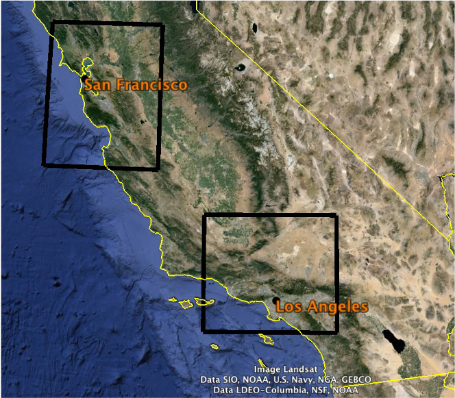
For this activity, you will use the historical seismicity to determine the probability of various-sized earthquakes occurring in specific areas over the next year, and over the next 30 years. The data came from https://earthquake.usgs.gov/earthquakes/search/
San Francisco area (done as class) |
Los Angeles area (done individually for your lab report) |
|
|---|---|---|
Latitude range |
36.25 - 38.75 \(^{\circ}\)N |
33.5-35.5 \(^{\circ}\)N |
Longitude range |
120.75 - 123.25 \(^{\circ}\)W |
116.75 - 119.75 \(^{\circ}\)W |
Date range |
01/01/1983 - 12/31/2012 |
01/01/1983 - 12/31/2012 |
Magnitude ranges |
2.0-2.9, 3.0-3.9, up to 9.0-9.9 |
1-1.9, 2.0-2.9, 3.0-3.9, up to 9.0-9.9 |
Depth range |
All |
All |
Data source |
United States Geologic Survey |
United States Geologic Survey |
Database |
Example : San Francisco Area
Magnitude range |
total # of earthquakes 1983-2012 (30 years) |
average # of earthquakes per year |
MRI (mean recurrence interval in years) |
One year probability of earthquake occurring |
One year probability of earthquake not occurring |
|---|---|---|---|---|---|
2.0-2.9 |
1716 |
57.20 |
0.017 |
1.000 |
0.000 |
3.0-3.9 |
1326 |
44.20 |
0.023 |
1.000 |
0.000 |
4.0-4.9 |
161 |
5.37 |
0.186 |
1.000 |
0.000 |
5.0-5.9 |
13 |
0.43 |
2.308 |
0.433 |
0.567 |
6.0-6.9 |
3 |
0.10 |
10.000 |
0.100 |
0.900 |
7.0-7.9 |
0 |
0.00 |
50 (extrapolated) |
0.020 (extrapolated) |
0.9800 (extrapolated) |
8.0-8.9 |
0 |
0.00 |
300 (extrapolated) |
0.0033 (extrapolated) |
0.9967 (extrapolated) |
9.0-9.9 |
0 |
0.00 |
1600 (extrapolated) |
0.0006 (extrapolated) |
0.9994 (extrapolated) |
import pandas as pd
earthquakes = pd.read_csv('Files/US_Earthquakes_1983-2012.zip')
earthquakes
| time | latitude | longitude | depth | mag | magType | nst | gap | dmin | rms | ... | updated | place | type | horizontalError | depthError | magError | magNst | status | locationSource | magSource | |
|---|---|---|---|---|---|---|---|---|---|---|---|---|---|---|---|---|---|---|---|---|---|
| 0 | 1983-01-01T01:32:35.610Z | 38.198000 | -118.488000 | 3.599 | 2.89 | ml | 0.0 | 247.30 | NaN | 0.8580 | ... | 2016-02-02T18:50:21.010Z | 38km SSE of Hawthorne, NV | earthquake | NaN | NaN | 0.018 | 4.0 | reviewed | ci | ci |
| 1 | 1983-01-01T02:17:55.930Z | 35.745500 | -117.722000 | 5.680 | 2.01 | mc | 20.0 | 53.00 | NaN | 0.1200 | ... | 2016-02-03T01:12:47.200Z | 14km NE of Inyokern, CA | earthquake | 0.28 | 1.27 | NaN | 17.0 | reviewed | ci | ci |
| 2 | 1983-01-01T03:56:55.920Z | 33.933333 | -118.812000 | 0.353 | 2.16 | mh | 21.0 | 194.00 | NaN | 0.2100 | ... | 2016-04-01T23:29:13.318Z | 8km S of Malibu, CA | earthquake | 0.85 | 1.05 | 0.309 | 11.0 | reviewed | ci | ci |
| 3 | 1983-01-01T04:03:54.690Z | 35.810000 | -117.735500 | 5.245 | 2.50 | ml | 31.0 | 60.00 | NaN | 0.1800 | ... | 2016-04-01T20:13:31.091Z | 19km NNE of Inyokern, CA | earthquake | 0.34 | 1.14 | 0.013 | 4.0 | reviewed | ci | ci |
| 4 | 1983-01-01T04:12:21.890Z | 35.816500 | -117.739000 | 4.979 | 2.85 | ml | 35.0 | 61.00 | NaN | 0.2100 | ... | 2016-04-02T12:24:09.816Z | 20km NNE of Inyokern, CA | earthquake | 0.40 | 1.07 | 0.202 | 10.0 | reviewed | ci | ci |
| ... | ... | ... | ... | ... | ... | ... | ... | ... | ... | ... | ... | ... | ... | ... | ... | ... | ... | ... | ... | ... | ... |
| 231157 | 2012-12-31T21:00:14.700Z | 34.914000 | -119.593000 | 7.565 | 2.43 | ml | 44.0 | 53.00 | 0.15010 | 0.2600 | ... | 2022-07-24T14:45:00.773Z | 24km SW of Maricopa, CA | earthquake | 0.38 | 0.86 | 0.160 | 67.0 | reviewed | ci | ci |
| 231158 | 2012-12-31T21:00:40.960Z | 37.637333 | -122.496833 | 8.540 | 2.11 | md | 97.0 | 93.00 | 0.01712 | 0.0800 | ... | 2022-07-24T14:43:42.150Z | 2 km NNW of Pacifica, California | earthquake | 0.14 | 0.18 | 0.152 | 63.0 | reviewed | nc | nc |
| 231159 | 2012-12-31T21:22:24.430Z | 40.434500 | -123.364833 | 28.967 | 2.42 | md | 33.0 | 33.00 | 0.08919 | 0.2100 | ... | 2017-01-29T05:39:58.660Z | 12 km E of Mad River, California | earthquake | 0.41 | 0.99 | 0.130 | 32.0 | reviewed | nc | nc |
| 231160 | 2012-12-31T22:36:06.070Z | 38.817833 | -122.798333 | 1.100 | 2.06 | md | 60.0 | 20.00 | 0.00991 | 0.0700 | ... | 2017-01-29T05:40:38.730Z | 6 km W of Cobb, California | earthquake | 0.10 | 0.18 | 0.142 | 31.0 | reviewed | nc | nc |
| 231161 | 2012-12-31T23:02:17.428Z | 38.716200 | -116.689600 | 0.000 | 2.10 | ml | 5.0 | 230.45 | 1.14800 | 0.2014 | ... | 2018-06-29T20:50:58.679Z | 63 km SSE of Kingston, Nevada | earthquake | NaN | 0.00 | 0.050 | 2.0 | reviewed | nn | nn |
231162 rows × 22 columns
The following lines show how to select earthquakes in a catalog that fall within a range of latitudes and longitudes (i.e. a box):
earthquakes.columns
Index(['time', 'latitude', 'longitude', 'depth', 'mag', 'magType', 'nst',
       'gap', 'dmin', 'rms', 'net', 'id', 'updated', 'place', 'type',
       'horizontalError', 'depthError', 'magError', 'magNst', 'status',
       'locationSource', 'magSource'],
      dtype='object')
earthquakes_san_francisco = earthquakes[(earthquakes.latitude > 36.25) & (earthquakes.latitude < 38.75) & (earthquakes.longitude > -123.25) & (earthquakes.longitude < 120.75)]
Now, we can select a range of magnitudes within this catalog:
len(earthquakes_san_francisco[(earthquakes_san_francisco.mag >= 3) & (earthquakes_san_francisco.mag < 4)])
5131
Let is make a Python function to do the filtering above, so that we can run these for various regions and magnitude ranges:
def catalog_filter(catalog, minlon=None, maxlon=None, minlat=None, maxlat=None, minmag = 0, maxmag = 10):
    if minlon==None or maxlon==None or minlat==None or maxlat==None:
        catalog_filtered = catalog[(catalog.mag >= minmag) & (catalog.mag < maxmag)]
    else:
        catalog_filtered = catalog[(catalog.latitude >= minlat) & (catalog.latitude <= maxlat) &
                               (catalog.longitude >= minlon) & (catalog.longitude <= maxlon) &
                               (catalog.mag >= minmag) & (catalog.mag < maxmag)
                              ]
    return catalog_filtered
earthquakes_san_francisco = catalog_filter(earthquakes, -123.25, -120.75, 36.25, 38.75)
earthquakes_los_angeles = catalog_filter(earthquakes, -119.75, -116.75, 33.5, 35.5)
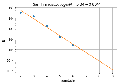
Question 2.1 The Gutenburg Richter Law is described as \(\log_{10}(N) = a - bM\) where \(N\) is the greater of Earthquake smaller than magnitude \(M\). In essence, this means that there is an exponentially higher likelihood of small versus large earthquakes. The \(b\) value is commonly close to 1.0 in seismically active regions. This means that for a given frequency of magnitude 4.0 or larger events there will be 10 times as many magnitude 3.0 or larger quakes and 100 times as many magnitude 2.0 or larger quakes.
If earthquakes in both San Francisco and Los Angeles follow the Gutenberg-Richter Law, report the \(b\) value in the two regions? Here are the number of earthquakes in Los Angeles for use:
Magnitude range |
total # of earthquakes 1983-2012 (30 years) |
|---|---|
1.0-1.9 |
76487 |
2.0-2.9 |
21471 |
3.0-3.9 |
1830 |
4.0-4.9 |
209 |
5.0-5.9 |
26 |
6.0-6.9 |
2 |
7.0-7.9 |
0 |
8.0-8.9 |
0 |
9.0-9.9 |
0 |
Hint: An example on how to do this for San Francisco is provided below.
# magnitude from the table (lower bound from each range)
M = np.arange(2,10)

# number of earthquakes for each magnitude range
n = np.array([1716,1326,161,13,3,0,0,0])

# number of earthquakes with magnitude greater than or equal to M
N = np.cumsum(n[::-1])[::-1]

# manual sum
#N = np.array([3219, 1503,  177,   16,    3,    0,    0,    0])

#Fit a straight line to find the parameter
p = np.polyfit(M[n>0], np.log10(N[n>0]), 1)
a = p[1]
b = -p[0]
N_fit = 10 ** (a - b * np.array(M))

import matplotlib.pyplot as plt
plt.figure()
plt.semilogy(M, N, 'o')
plt.plot(M, N_fit)
plt.title('San Francisco: $log_{10}N = %.2f - %.2f M$' % (a, b))
plt.xlabel('magnitude')
plt.ylabel('N')
plt.grid()
plt.show()
Answer:
Question 2.2 Note the slight deviation at small magnitudes (~2-3) to fewer than expected detections of small earthquakes. This kink is indicative of something called the magnitude of completeness of a seismicity catalog, a threshold magnitude below which not all earthquakes may be detected. This bias can be accounted for by excluding earthquakes below the magnitude of completeness while estimate the \(b\) value (which we will leave to the experts for now!). Why are smaller earthquakes harder to detect? Hint: Think signal-to-noise ratio (SNR).
Answer:
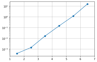
Question 2.3 Fill the table of joint probabilities of earthquakes happening within a 30-year period for the Los Angeles Area based on the instructions below:
First two columns are provided. The values were calculated for you by using the
catalog_filterfunction.Calculate the average number of earthquakes per year that occurred in each magnitude range.
Calculate the mean recurrence interval (MRI) for each magnitude range up through magnitude 6.0-6.9. The MRI is defined as the average time between earthquakes. Extrapolate MRI for magnitude 7.0 or above (see hint below).
Determine the probability of earthquakes of each magnitude range occurring in one year, expressed as either a fractional probability between 0 and 1.0.
For earthquakes with MRI’s greater than one year: Fractional probability = 1/ MRI and then multiply by 100 to get % probability. (Note that this is equal to the average # of earthquakes per year. But using the 1/ MRI method allows calculation of probabilities for earthquakes that haven’t occurred over the study period - because we have extrapolated MRI’s.)
Determine the probability of each earthquake magnitude NOT occurring in a year. This will simply be is 1.0 minus the probability of that thing occurring in a year.
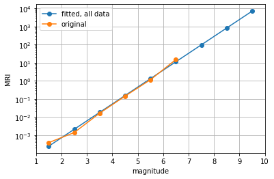
Hint: How to extrapolate MRI:
Plot MRI as a function of magnitude to see the relationship. You will find that MRI is an exponential function of magnitude
Fit a straight line \(\log_{10}(\text{MRI}) = intercept + slope * M\) where \(M\) is the magnitude
Use \(intercept\) and \(slope\) to calculate MRI for magnitude range 7.0-7.9, 8.0-8.9, and 9.0-9.9.
# the centers of the magnitude ranges
mag = np.array([1.5,2.5,3.5,4.5,5.5,6.5,7.5,8.5,9.5])

# number of earthquakes over 30 years
n = np.array([76487,21471,1830,209,26,2,0,0,0])

# Mean recurrence intervals in years
MRI = 30/n

# notice that the last 3 elements are inf
MRI
/tmp/ipykernel_130801/4143073906.py:8: RuntimeWarning:

divide by zero encountered in true_divide
array([3.92223515e-04, 1.39723348e-03, 1.63934426e-02, 1.43540670e-01,
       1.15384615e+00, 1.50000000e+01,            inf,            inf,
                  inf])
MRI_valid = MRI[MRI < np.inf]
mag_valid = mag[MRI < np.inf]

plt.semilogy(mag_valid, MRI_valid, '-o')
plt.xlim(1,7)
plt.grid()
plt.show()
# fit log10(MRI) = a + b * magnitude
MRI_log = np.log10(MRI_valid)

p = np.polyfit(mag_valid, MRI_log, 1)
intercept = p[1]
slope = p[0]
MRI_fit = 10 ** (intercept + slope * mag)
plt.semilogy(mag, MRI_fit, '-o', label='fitted, all data')
plt.semilogy(mag_valid, MRI_valid, '-o', label='original')
plt.xlim(1,10)
plt.grid()
plt.legend()
plt.xlabel('magnitude')
plt.ylabel('MRI')
plt.show()
Answer:
Magnitude range |
total # of earthquakes 1983-2012 (30 years) |
average # of earthquakes per year |
MRI (mean recurrence interval in years) |
One year probability of earthquake occurring |
One year probability of earthquake not occurring |
|---|---|---|---|---|---|
1.0-1.9 |
76487 |
||||
2.0-2.9 |
21471 |
||||
3.0-3.9 |
1830 |
||||
4.0-4.9 |
209 |
||||
5.0-5.9 |
26 |
||||
6.0-6.9 |
2 |
||||
7.0-7.9 |
0 |
||||
8.0-8.9 |
0 |
||||
9.0-9.9 |
0 |
Question 2.4 Find the probability of a magnitude 7.0-7.9 earthquake occurring in the San Francisco in the next year – the annual probability of event. Compare that to the annual probability in Los Angeles.
Answer:
Question 2.5 Not a very high probability, perhaps, but then a year isn’t very long! Let’s say you are living in the Los Angeles area and take out a 30-year mortgage on a house. What is the probability of a magnitude 7.0-7.9 earthquake occurring during that 30-year period? How does this value compare to the probability of such an earthquake occurring in the San Francisco area in the next 30 years? Hint: You can modify the code for calculating the joint probability for San Francisco as provided below:
MRI = 50
num_years = 30
prob = (1 - (1 - 1/MRI) ** num_years)*100
print("Probability of a magnitude 7.0-7.9 earthquake occurring in the San Francisco are during that 30-year period is %.2f percent."%(prob))
Probability of a magnitude 7.0-7.9 earthquake occurring in the San Francisco are during that 30-year period is 45.45 percent.
Answer:
Mini-tutorial#
Mean and Standard Deviation with numpy
Statistical distributions and confidence intervals
Consider a set of observations \(x_i\) from \(i = 1\) to \(N\). The mean observation is denoted by \(\bar{x}\) and is obtained by summing all observations \(x_i\) and dividing by the number of observation \(N\):
The equation can be read as: For each of the \(N\) observations, calculate the deviation of the observation from the calculated mean. Square all of these deviations and sum them. Divide this sum by the total number of observations \(N\) minus one. Finally, take the square root of this number to arrive at the standard deviation \(\sigma\).
from scipy import stats, optimize, special, integrate
import numpy as np
import matplotlib.pyplot as plt
x = np.array([2, 3, 5, 10, 15])
print("x    =", x)
print("mean = {:.2f}".format(np.mean(x)))
print("std  = {:.2f}".format(np.std(x)))
x    = [ 2  3  5 10 15]
mean = 7.00
std  = 4.86
Once you know the mean \(\bar{x}\) and standard deviation \(\sigma\) of a normal distribution, you can define the probability distribution that describes the probability of obtaining a measurement in a certain range of \(x\). Note that all probability distributions have unit area such that \(\int_{-\infty}^{\infty} P(x)\) = 1. The probability distribution is a curve that can be described mathematically by the formula
In this formula, \(P(x)\) does not represent the probability of observing exactly \(x\). Instead, \(P(x)\) is called a probability density function, and the probability of observing a value between two arbitrary values \(a\) and \(b\) is the area beneath the curve in the range \([a, b]\) (meaning ‘a to b’ with both values included). For example, the probability that the next observation x lies between the mean minus one standard deviation and the mean plus one standard deviation (between \(\bar{x}-\sigma\) and \(\bar{x}+\sigma)\) is simply the area beneath \(P(x)\) over the interval \([\bar{x}-\sigma, \bar{x}+\sigma]\). This area turns out to be 0.68. Since 0.68 = 68%, you can also express this result as: we are 68% confident that the measurement will lie between \(\bar{x}-\sigma\) and \(\bar{x}+\sigma\).
It is important to remember that quite often, we do not actually observe the normal distribution. We collect a sample (usually not that large) and calculate the mean and the standard deviation. We then make the assumption that the underlying population has a normal distribution. This is not always true. When only a small number of measurements from a sample are used to estimate \(\bar{x}\) and \(\sigma\) of the entire population, these numbers are less certain. In such cases, the probability distribution is more accurately described by Student’s t-distribution, which takes into account the uncertainties in \(\bar{x}\) and \(\sigma\) as well due to the limited sampling. Basically, this uncertainty will act to spread out the normal distribution when only few observations are used, since we are less certain about the distribution.
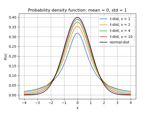
The probability distribution of a Student’s t-distribution is a curve that has unit area and is described mathematically by the formula:
where \(\nu\) is the degree of freedom (number of samples minus one), \(\bar{x}\) is the sample mean, \(\sigma\) is the sample standard deviation, and \(\Gamma(z) = (z - 1)!\) (see the gamma function).
The example below illustrates how samples are generated from a Normal distribution with known population mean and population standard deviation. When you answer the questions below, you will be supplied with the data (treated as samples) without any knowledge of the underlying population mean and population standard deviation.
popmean,popstd = 30, 12
N = 5
#s = np.random.normal(popmean, popstd)
s = np.array([49.30996753, 20.97160251, 40.41776131, 18.44689402, 44.1202185 ]) # one random output from the command above
s
array([49.30996753, 20.97160251, 40.41776131, 18.44689402, 44.1202185 ])
Let’s pretend we do not know the population mean and the population standard deviation, and then we calculate the sample mean and the sample standard deviation.
samplemean = np.mean(s)
samplestd  = np.std(s)

print("Sample size    N = %d" % N)
print("Sample mean      = %.2f" % samplemean)
print("Sample std       = %.2f" % samplestd)
Sample size    N = 5
Sample mean      = 34.65
Sample std       = 12.55
Now, we will construct the probability density of the Student’s t-distribution from the *sample mean, the sample standard deviation, and the sample size using the function below.
def tdist_probability_density(x, dof, mean, std):
    '''
    Compute the probability density of the Student's t-distribution

    Input Parameters:
    ----------------

    x:         (array of) location(s) where the probability density is computed
    dof:       degree of freedom; equals to the sample size minus one
    mean:      sample mean
    std:       sample standard deviation

    Return:
    ------

    p:         probability density at all given x

    '''
    p = special.gamma((dof + 1) / 2) / special.gamma(dof / 2) / np.sqrt(np.pi * dof * std ** 2) * \
        (1 + (x - mean) ** 2 / std ** 2 / dof) ** (-(dof + 1) / 2)
    return p

def ndist_probability_density(x, mean, std):
    '''
    Compute the probability density of the Normal distribution

    Input Parameters:
    ----------------

    x:         (array of) location(s) where the probability density is computed
    mean:      sample mean
    std:       sample standard deviation

    Return:
    ------

    p:         probability density at all given x

    '''
    p = np.exp(-1/2 * (x - mean) ** 2  / std ** 2) / np.sqrt(2 * np.pi * std ** 2)
    return p
The cumulative density function (CDF) is obtained by integrating the probability density function from \(-\infty\) to \(x\).
def tdist_cumulative_density(x, dof, mean, std):
    '''
    Compute the cumulative density of the Student's t-distribution

    Input Parameters:
    ----------------

    x:         (array of) location(s) where the probability density is computed
    dof:       degree of freedom; equals to the sample size minus one
    mean:      sample mean
    std:       sample standard deviation

    Return:
    ------

    c:         cumulative density at all given x

    '''
    c = integrate.quad(tdist_probability_density, -np.inf, x, args=(dof, mean, std))[0]
    return c

def ndist_cumulative_density(x, mean, std):
    '''
    Compute the cumulative density of the Normal distribution

    Input Parameters:
    ----------------

    x:         (array of) location(s) where the probability density is computed
    mean:      sample mean
    std:       sample standard deviation

    Return:
    ------

    c:         cumulative density at all given x

    '''
    c = integrate.quad(ndist_probability_density, -np.inf, x, args=(mean, std))[0]
    return c
Here is how to calculate the value such that there is a 95% chance that a sample drawn from the Student’s t-distribution is smaller
def find_confidence_interval_onesided(dof, mean, std, prob, distribution='t'):
    '''
    Computes the value to give any probability that a sample draw from
    the Student's t-distribution is smaller than this value. In other words,
    this function finds the value such that CDF(value | dof, mean, std) = prob.

    Input Parameters:
    ----------------

    dof:       degree of freedom; equals to the sample size minus one
    mean:      sample mean
    std:       sample standard deviation
    prob:      target probability
    distribution:    which type of distribution ('t' or 'normal')

    Return:
    ------

    value:     a value such that CDF(value) = prob

    '''
    # function to optimize
    # which is the difference between the cumulative distribution and target probability
    if distribution == 't':
        def func_to_optimize(x, dof, mean, std, prob):
            return tdist_cumulative_density(x, dof, mean, std) - prob
    else:
        def func_to_optimize(x, dof, mean, std, prob):
            return ndist_cumulative_density(x, mean, std) - prob

    # x0 and x1 are initial and second guesses
    value = optimize.root_scalar(func_to_optimize, args=(dof, mean, std, prob), x0=mean, x1=mean+std).root
    return value
find_confidence_interval_onesided(N-1, samplemean, samplestd, 0.95) # 95% == 0.95
61.407853899787334
P = 0.005
find_confidence_interval_onesided(N-1, 0, 1, 1-P)
4.604094871350386
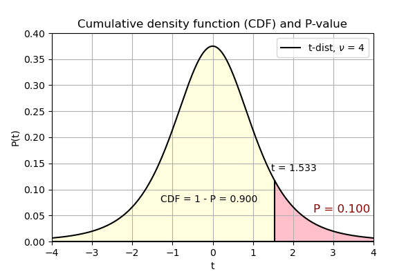
Values of \(t\) score (\(t = \frac{x - \bar{x}}{\sigma}\)) corresponding to given values of \(P\) and \(\nu\) degree of freedom are provided in the table below. The value \(P\) is defined as the area under the probability density curve to the right of \(t\). The area under the probability density curve to the left is the cumulative density function. The value corresponding to the figure below is marked in bold inside the table.
Degree of freedom \(\nu\) |
P=0.005 |
P=0.01 |
P=0.025 |
P=0.05 |
P=0.10 |
P=0.25 |
|---|---|---|---|---|---|---|
1 |
63.657 |
31.281 |
12.706 |
6.314 |
3.078 |
1.000 |
2 |
9.925 |
6.945 |
4.303 |
2.920 |
1.886 |
0.816 |
3 |
5.841 |
4.541 |
3.182 |
2.353 |
1.638 |
0.765 |
4 |
4.604 |
3.747 |
2.776 |
2.132 |
1.533 |
0.741 |
5 |
4.032 |
3.365 |
2.571 |
2.015 |
1.476 |
0.727 |
6 |
3.707 |
3.143 |
2.447 |
1.943 |
1.440 |
0.718 |
7 |
3.499 |
2.998 |
2.365 |
1.895 |
1.415 |
0.711 |
8 |
3.355 |
2.896 |
2.306 |
1.860 |
1.397 |
0.706 |
9 |
3.250 |
2.821 |
2.262 |
1.833 |
1.383 |
0.703 |
10 |
3.169 |
2.764 |
2.228 |
1.812 |
1.372 |
0.700 |
15 |
2.947 |
2.602 |
2.131 |
1.753 |
1.341 |
0.691 |
20 |
2.845 |
2.528 |
2.086 |
1.725 |
1.325 |
0.687 |
25 |
2.787 |
2.485 |
2.060 |
1.708 |
1.316 |
0.684 |
30 |
2.750 |
2.457 |
2.042 |
1.697 |
1.310 |
0.683 |
\(\infty\) |
2.576 |
2.326 |
1.960 |
1.645 |
1.282 |
0.674 |
Part III: The Parkfield Prediction#
It is important to realize that the general observation that earthquakes recur on individual faults can be the result of many physical realities. The simple ‘sawtooth’ earthquake cycle model may be attractive because of its simplicity, but its validity has to be confirmed by observational data. This model has come under a great deal of criticism lately, because its predictions for the locations of earthquakes over the past 20 years along the Pacific rim have not been very successful.

The purpose of this problem is to illustrate how probabilistic forecasts are made by calculating the likely time for next Parkfield earthquake using statistics.
Background: The National Earthquake Prediction Evaluation Council (NEPEC) in 1985 endorsed a prediction that with 95% confidence (= probability), the next Parkfield earthquake would occur before January 1993.
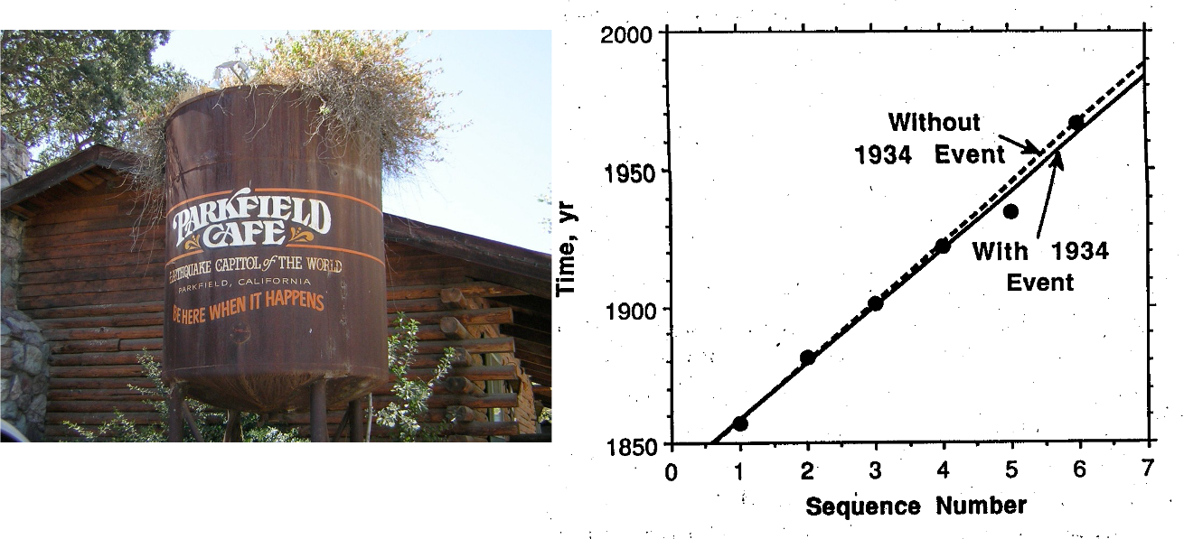
The Data: At the time, most seismologists agreed that earthquakes of very similar size and character (that is, which ruptured the same part of the San Andreas Fault) have occurred near Parkfield at the following times: 1857, 1881, 1901, 1922, 1934, and 1966. There is no record of earthquake activity before 1857, but we do not expect there to be one because the area was not settled at that time.
In order to calculate expectations and probabilities, you have to have a model in mind which tells you what the data above represent. It is not clear which model is most appropriate, and you may think of a better one than the following:
Approach 1 — strictly numbers. The sequence clearly suggests a repetition with approximately the same interval between events. If we think of the intervals between earthquakes as belonging to a normal distribution with some mean, the data can be used to estimate both an average repeat time and a standard deviation around that mean.
Question 3.1 Calculate the mean value and the standard deviation for the earthquake repeat times. Hint: Create a numpy array for years = np.array([1857, 1881, 1901, 1922, 1934, 1966]) and use standard numpy functions.
Answer:
Question 3.2 Based on the values derived above, what is the predicted (i.e. most likely) time for an earthquake to occur following the 1966 earthquake ?
Answer:
Question 3.3 What is the time before which there is a 95% probability that the earthquake will occur? Hint: Since there are very few observations, you need to know something about Student’s t-distributions to answer this question. See mini-tutorial above.
Answer:
Approach 2 — using some ‘insights’. Assume that the 1934 earthquake really should have occurred in 1944, but that it for some reason was ‘triggered’ to occur prematurely by some other geophysical process.
Question 3.4 Repeat the analysis for mean and standard deviation but assume that the 1934 event really occurred in 1944.
Answer:
Question 3.5 Which approach appears to be closest to the one used by the NEPEC? If we were uncertain about the correctness of different approaches to interpreting the data (for example Approaches 1 and 2 above) how might one incorporate these uncertainties in the probability estimates?
Answer:
Question 3.6 The long-awaited Parkfield earthquake finally occurred on September 28, 2004! Include the 2004 data point to
(a) Re-calculate the mean value and standard deviation for the earthquake repeat time with this year.
(b) Predict the year for the next Parkfield earthquake with 95 % probability.
Answer: