GeoExchange Site Visit and Local Geology Field Trip

IN THE SPACE BELOW, WRITE OUT IN FULL AND THEN SIGN THE HONOR PLEDGE:

“I pledge my honor that I have not violated the honor code during this examination.”

PRINT NAME:

If a fellow student has contributed significantly to this work, please acknowledge them here:

Peer(s):

Contribution:

By uploading this assignment through Canvas, I sign off on the document below electronically.

---

Part I: Geotherm: Temperature within the Earth

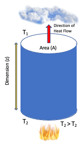
Conduction is the process by which heat is transferred from the hotter end to the colder end of an object. The ability of the object of dimension \(z\) to conduct heat is known as its thermal conductivity, and is denoted \(k\). Heat spontaneously flows along a temperature gradient \(\nabla\)T = (T₂-T₁)/\(z\), a physical quantity that describes in which direction and at what rate the temperature changes the most rapidly around a particular location. Fourier’s Law of heat conduction is expresses the flux or the rate of heat flow (\(Q\) in \(mW/m^2\)) as:

\[ Q = k \cdot A \frac{T_2-T_1}{z}, \]

where the symbols and their typical values are provided in the table below.

The expressions below is a model calculating an approximate conductive geothermal gradient for the lithosphere. Note that these have been derived by taking a cylinder rock of length \(z\) and area \(A\) and considering Fourier’s Law. Also provided is a code snippet to plot the geotherm interactively. Your task is to experiment with and comment on this model by changing parameters (e.g. mantle heat flow, thermal conductivity). We explore this in the questions below. Note that the thermal conductivities are derived from samples at room temperature (refer Pollack et al., Journal of Geophysical Research, 1993). In the real Earth, some of these properties can vary both with depth (e.g. \(k\)) and location on the surface (e.f. T\(_s\)).

\[\begin{split} \mathrm{T}(z) = \begin{cases} \frac{Qz}{K}+\frac{A_\mathrm{o}z(b-z/2)}{K} +T_s & \text{if } z < b \\ % & is your "\tab"-like command (it's a tab alignment character) \frac{Qz}{K}+\frac{A_\mathrm{o}b^2}{2K} +T_s & \text{b $\leq$ z $\leq$ L, where L = 100 km } \end{cases} \end{split}\]

Parameter	Symbol	Typical Value	Units
Temperature at the surface	T\(_s\)	15	\(^{\circ}\)C
Heat flow in continents	Q	65	mW/m\(^2\)
Heat flow in oceans	Q	101	mW/m\(^2\)
Thermal conductivity of Granite	k	3.1	W/m/deg
Thermal conductiity of Basalt	k	1.5	W/m/deg
Heat production	A\(_\mathrm{o}\) = \(\rho\)H\(_s\)	2.0	\(\mu\)W/m\(^3\)
Characteristic depth of A\(_\mathrm{o}\)	b	10	km
Depth	z	Variable	km

# import packages
import pandas as pd
import numpy as np
import plotly.express as px
import plotly.graph_objects as go

# Define constants
Ts = 15
Q = 65
Ao = 2
b = 10
K = 3.1
L = 100 #km

# create dataframe
z = np.arange(0,L+1)
df = pd.DataFrame({'Depth (km)': z})
  
#adding column with constant value
# Note that in the Earth, this might vary with location
df['Q'] = pd.Series([Q for x in range(len(df.index))])
df['Ao'] = pd.Series([Ao for x in range(len(df.index))])
df['K'] = pd.Series([K for x in range(len(df.index))])
    
# view dataframe
#print("Initial dataframe")
#display(df)

df.loc[df['Depth (km)'] < b, 'T (Centigrade)'] = df['Q']*df['Depth (km)']/df['K'] + df['Ao']*df['Depth (km)']*(b-df['Depth (km)']/2)/df['K'] + Ts
df.loc[(df['Depth (km)'] >= b) & (df['Depth (km)'] <= L), 'T (Centigrade)'] = df['Q']*df['Depth (km)']/df['K'] + df['Ao']*b**2/(2*df['K']) + Ts

# flipped the depth 
fig1 = px.line(df, x="T (Centigrade)", y="Depth (km)")
fig = go.Figure(data=fig1.data, layout = fig1.layout)
fig.update_layout(
    yaxis = dict(autorange="reversed"),
    title_text='Conductive geotherm in continents',
    width=400, height=500
)
fig.show()

TO DO

Question 1.1. What is the temperature at the base of the continental crust? Assume average thickness globally across all continents to be 40 km.

Answer:

Question 1.2. (A) Play around with the parameters of the model. What do you need to do to get 700\(^{\circ}\) at the base of the continental crust? Make a interactive plot like the one above for your favorite scenario. (B) Is there a unique solution? Which parameters do you think we know best? the least?

Answer:

Question 1.3.(A) The typical values of heat flux from the oceans are much higher (see table). Plot the conductive geotherm for the oceanic lithosphere by modfying the code above with the relevant constants. (B) Report the temperature at depths corresponding to Question 1.1. Is it higher or lower? © Speculate on the reasons why heat flow is higher in oceans versus continents? Hint: think about structural differences between the two and what happends near a mid-ocean ridge.

Answer:

Question 1.4. The equations given above assume that heat flow in the lithosphere is by conduction only. Is this a reasonable assumption? Why or why not?

Answer:

Part II: GeoExchange Site at Princeton

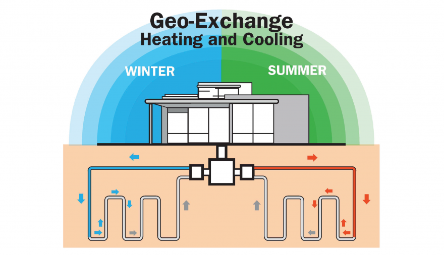
Princeton University needs heating and cooling around the year. In the winter, buildings are heated with steam. In the summer, they are cooled with chilled water. But, even on the coldest winter days, Princeton still needs to remove heat from the campus to cool lasers, electron microscopes, CT scan machines, computer facilities, and some building cores. And, even on the hottest summer days, Princeton needs to deliver heat to the campus for domestic hot water, dish washing, sterilizers, autoclaves, cage washers, and air‐conditioning reheat for humidity control and comfort. There is a sizable need for simultaneous heating and cooling all year.

import pandas as pd
PU_Data = pd.read_excel('Files/Microgrid_PU_Data_8-31-2022.xlsx')

PU_Data

	Timestamp	Campus Total Cooling Demand, Tons	Outdoor Air Temperature, F	Total Campus Steam Demand, Pounds Per Hour	Total Campus Power Demand, KW	Locational Marginal Price, $/MWH
0	2020-07-01 00:00:00	6465.366	71.039	36663.306	12531.491	14.123596
1	2020-07-01 01:00:00	6457.861	69.605	36743.513	12325.745	15.380625
2	2020-07-01 02:00:00	6240.119	69.600	36930.052	12195.363	14.876885
3	2020-07-01 03:00:00	6126.111	69.286	36897.495	12146.217	14.004767
4	2020-07-01 04:00:00	5553.196	69.176	36063.303	12201.516	13.325767
...	...	...	...	...	...	...
17513	2022-06-30 20:00:00	6061.833	86.258	37043.694	17035.897	78.367859
17514	2022-06-30 21:00:00	5699.684	83.177	35135.220	17048.291	52.693565
17515	2022-06-30 22:00:00	5700.993	79.999	35613.224	16987.258	60.326447
17516	2022-06-30 23:00:00	5056.392	76.292	35493.236	16242.035	56.912426
17517	2022-07-01 00:00:00	3258.427	75.782	20110.547	15781.712	58.150692

17518 rows × 6 columns

PU_Data.info()

<class 'pandas.core.frame.DataFrame'>
RangeIndex: 17518 entries, 0 to 17517
Data columns (total 6 columns):
 #   Column                                      Non-Null Count  Dtype         
---  ------                                      --------------  -----         
 0   Timestamp                                   17518 non-null  datetime64[ns]
 1   Campus Total Cooling Demand, Tons           17518 non-null  float64       
 2   Outdoor Air Temperature, F                  17518 non-null  float64       
 3   Total Campus Steam Demand, Pounds Per Hour  17518 non-null  float64       
 4   Total Campus Power Demand, KW               17517 non-null  float64       
 5   Locational Marginal Price, $/MWH            17518 non-null  float64       
dtypes: datetime64[ns](1), float64(5)
memory usage: 821.3 KB

• Btu delivered per pound of steam : 950

• 1 Btu = 3,412 KWH

• Btu removed per Ton-Hour during cooling : 12,000

• Assuming heating system is 80% efficient. Building heat addition is less than heating energy requirements in the system specifications due to inefficiencies.

PU_Data['Campus building heat addition, MW']=PU_Data['Total Campus Steam Demand, Pounds Per Hour']*950/3412/1000*0.8

PU_Data['Campus heat removal, MW'] = PU_Data['Campus Total Cooling Demand, Tons']*12000/3412/1000

PU_Data

	Timestamp	Campus Total Cooling Demand, Tons	Outdoor Air Temperature, F	Total Campus Steam Demand, Pounds Per Hour	Total Campus Power Demand, KW	Locational Marginal Price, $/MWH	Campus building heat addition, MW	Campus heat removal, MW
0	2020-07-01 00:00:00	6465.366	71.039	36663.306	12531.491	14.123596	8.166504	22.738685
1	2020-07-01 01:00:00	6457.861	69.605	36743.513	12325.745	15.380625	8.184370	22.712290
2	2020-07-01 02:00:00	6240.119	69.600	36930.052	12195.363	14.876885	8.225920	21.946491
3	2020-07-01 03:00:00	6126.111	69.286	36897.495	12146.217	14.004767	8.218668	21.545525
4	2020-07-01 04:00:00	5553.196	69.176	36063.303	12201.516	13.325767	8.032858	19.530584
...	...	...	...	...	...	...	...	...
17513	2022-06-30 20:00:00	6061.833	86.258	37043.694	17035.897	78.367859	8.251233	21.319460
17514	2022-06-30 21:00:00	5699.684	83.177	35135.220	17048.291	52.693565	7.826133	20.045782
17515	2022-06-30 22:00:00	5700.993	79.999	35613.224	16987.258	60.326447	7.932606	20.050386
17516	2022-06-30 23:00:00	5056.392	76.292	35493.236	16242.035	56.912426	7.905879	17.783325
17517	2022-07-01 00:00:00	3258.427	75.782	20110.547	15781.712	58.150692	4.479489	11.459884

17518 rows × 8 columns

Princeton will use big tanks of hot and cold water and big geoexchange borefields for thermal energy storage. The thermal storage tanks hold a few million gallons each; large enough to deliver heating or cooling for several hours. The geoexchange wellfields are large enough to store an entire heating season of energy for the campus! Typical geoexchange wellfields include hundreds of wells. We’re now drilling over a thousand geoexchange bores on campus, each 850 feet deep and each placed in a grid pattern spaced 20 feet apart. We’re installing a 1.5‐inch‐diameter U‐bend of HDPE plastic tube in each bore and grouting it in place for its entire depth. When we pump warm water from the heat pumps’ condensers down through the HDPE tubes, it will give up its heat through the grout into the surrounding rock. The rock under our campus at that depth is naturally 50‐55 degrees Fahrenheit, so water entering at 90 degrees will give up its heat to the rock and return to the surface at 60‐70 degrees. The earth becomes a heat sink all summer long. Over the course of the summer the rock gradually heats up, acting as a seasonal energy storage reservoir. We will harvest heat from campus buildings all summer, preserve it for several months underground, and reclaim much of it in winter. Some heat will dissipate through the surrounding rock, but billions of pounds of warm rock will store an ample supply of heat that can be moved back to campus when it’s needed.

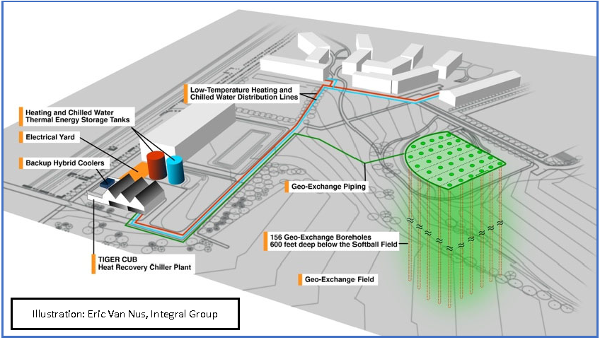
Figure: Princeton’s district energy expansion project will include the use of bore holes situated beneath the university’s softball field, new buildings, and other campus spaces. The illustration here captures the essence of the geoexchange component. Source: Princeton Geo-Exchange

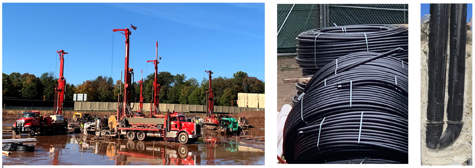
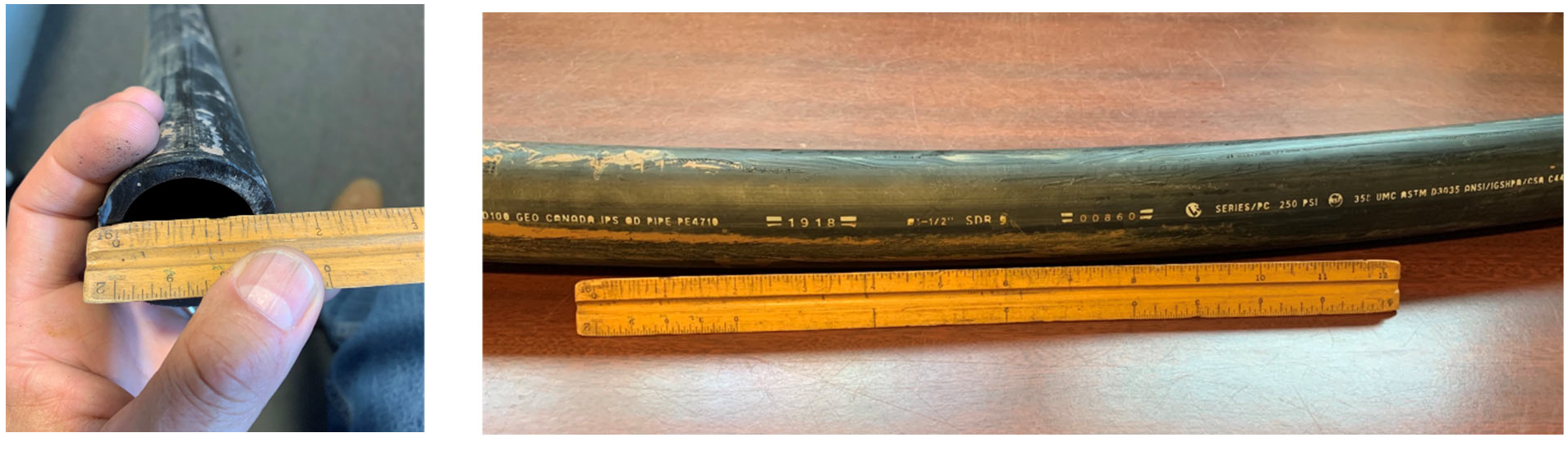
Figure: Princeton is installing over a thousand geoexchange bores on campus. The bores are between 600 and 850 feet deep. 1.5 inch diameter HDPE tube is inserted in the wells in a U‐bend to carry water down to the bottom and back to the surface again. As the water is pumped through the wells it will give up heat to the rock (summer) or pick up heat from the rock (winter). Source: Princeton Geo-Exchange

TO DO

Question 2.1. (a) Based on the interactive plot on energy usage, what is the peak heating need on the Princeton University campus? (b) What is the peak cooling need? © How much simultaneous heating and cooling is needed i.e. how much heating energy could be produced by the heat that is concurrently being removed in the process of cooling the campus?

Answer:

Question 2.2. The following exercises consider whether an entire season of heat removed from campus could be stored in geoexchange wells below campus. Each of these calculations is simplified to demonstrate the general concept of campus‐scale seasonal energy storage.

(A) Assume a rectangular geoexchange wellfield where the geoexchange wells are spaced in a grid pattern 20 feet from center‐to‐center and the geoexchange wells extend down 850 feet in the rock below campus. How many cubic feet of rock are associated with each geoexchange well? If the average density of rock is 165 pounds per cubic foot and there are 1000 wells in the geoexchange field, how many pounds of rock are associated with the wellfield?

(B) The total amount of heat removed from campus in a year from cooling is 418 billion Btu. How much heat energy would each pound of rock need to store to hold an entire year of heat removed from the campus?

© Assume the specific heat of rock is 0.47 Btu/pound/degree F. How many degrees will the rock in the Geoexchange array rise if an entire season of heat is stored?

Answer:

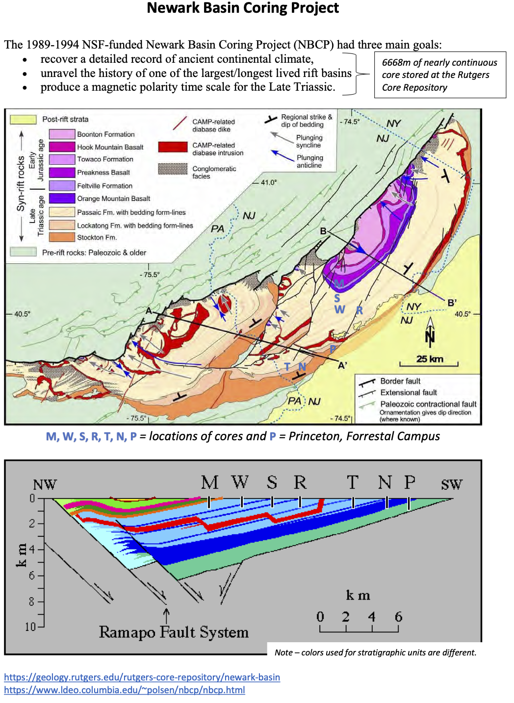
Newark Basin Coring Project

The Newark Basin Coring Project (NBCP) was a scientific drilling project funded by the National Science Foundation from 1989 to 1994. The three main goals of the project were to recover a very long and detailed record of ancient continental climate, unravel the history of one of the largest and longest lived rift basins, and produce a magnetic polarity time scale for the Late Triassic. The lcoations of wells in the southern Newark Basin are plotted below. Because of the tilt of the strata, a series of relatively shallow cores could be drilled, with overlapping geometries, in order to get a very detailed record of the stratigraphy of the entire basin. Three main goals of the project are described, and details of the project can be found at Rutgers University. The importance of archiving such records and making them available for research is critical to the ongoing process of science. More than 25 years after the cores were retrieved, they continue to provide insights in to Earth history.

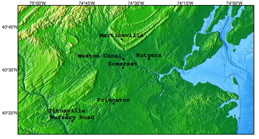
The locations of wells in the southern Newark basin near Princeton are provided in the map below.

TO DO

Question 2.3. Based on the location of the Princeton hole (40°22’09”N, 74°36’49”W), what formation did the Newark Basin Coring Project start drill at on the surface? What formations should it have expected to encounter based on the geological map and cross-sections above?

Answer:

Question 2.4. More that 36 years later, when the contractors for the GeoExchange project at Princeton University started drilling on and near the Princeton University campus. The reported descriptions of samples called tailings from the boreholes on campus indicated that the formation consisted of silty clay, shale, and sandstone. A log of one of the boreholes is provided below. Are these properties of this unit, which you identified in Question 3.3, consistent with your knowledge of the formation (feel free to add notes from the Rockd App)? Using your understanding of the compactness (or porosity) of the rock types, how will fluid circulation in this formation influence your estimated heat storage properties in Question 2.2?

Tailing description	Depth (feet)
Brown silty clay	0’-9’
Red shale	9’-15’
Grey sandstone	15’-19’
Red shale	19’-111’
Grey sandstone	111’-131’
Red shale	131’-170’
Grey sandstone	170’-420’
Red shale	420’-450’
Grey sandstone	450’-580’
Red shale	580’-625’
Grey sandstone	625’-660’
Red shale	660’-850’

Answer:

Geophysical Well Logs

Thousands of holes are drilled every year throughout the world, ranging from a few metres deep for engineering purposes, to over 14 km in the Kola Peninsula of northeast Russia, drilled to investigate the crust at depth. Drilling is usually done using a rotating bit that grinds away the formations to produce cuttings such as from shales and sand from unconsolidated sandstones. The variation of a property down a borehole is recorded against depth as a log.

Geophysical measurements are made by sophisticated instruments suspended by a wire, as they are pulled to the surface by a winch fitted with a depth counter. The instruments are called sondes or tools, and the measurements they produce are known variously as wire-line logs, geophysical well logs, or simply well logs.Well logging differs from most other geophysical methods, not only in being carried out down a borehole, but in relating the physical quantities measured more specifically to geological properties of interest, such as lithology, porosity, and fluid composition. Here is an example from the Newark Basin Coring Project from the Princeton borehole.

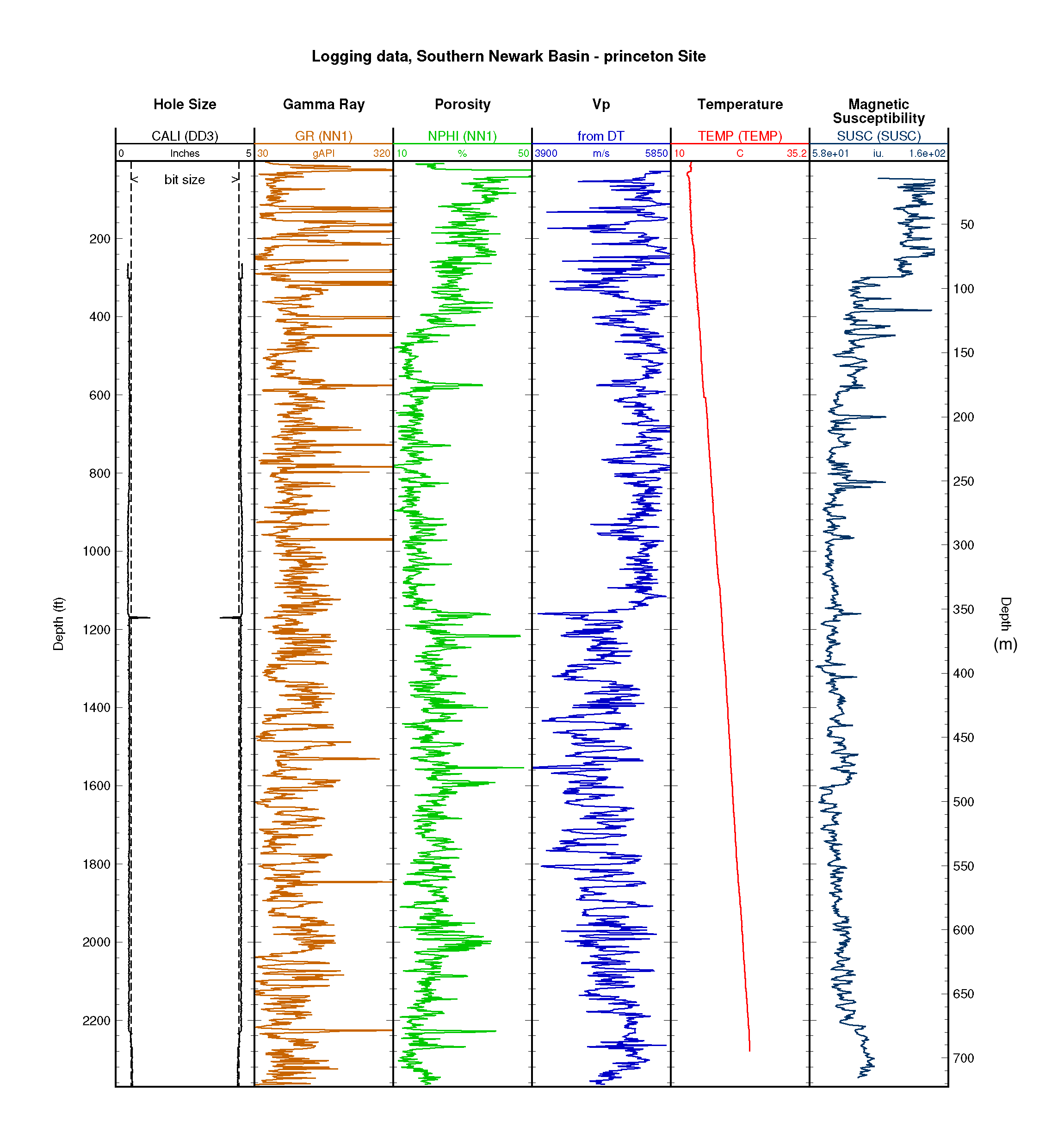
*Figure: Princeton hole at (40°22’09”N, 74°36’49”W) from Newark Basin Coring Project. Data accessed from Borehole Research Group of the Lamont-Doherty Earth Observatory of Columbia University.

TO DO

Question 2.5. Based on this well log from the Newark Basin Coring project, at what depth beneath the Princeton area do you expect to see a change in physical properties like porosity and compressional-wave velocity (\(v_P\))? Name the formation units you expect above and below this boundary. Hint: It is deeper than 100 m.

Answer:

Part II: Local Geology Outcrops

Installations: Please install the following apps on your smartphones:

• Rockd

• Fieldmove-clino

  • Fieldmove-clino for iOS

  • Fieldmove-clino for Android

Geological mapping of the region and boreholes drilled into the subsurface have revealed unprecendented insights into the stratigraphic formations in the subsurface. The Newark basin is perhaps the most extensively studied of the early Mesozoic basins of eastern North America that formed during the breakup of Pangea. The basin is around 190 km long and a maximum of 50 km wide. In general terms, the basin is bounded on its northwestern and northern margins by a system of mostly normal border faults. Along the southeastern and southern margins, Mesozoic rocks rest unconformably on Precambrian and Paleozoic basement rocks; in places, Mesozoic rocks are buried by Cretaceous coastal-plain strata. Although disrupted by intrabasinal faults and warped by transverse folds developed in the hanging walls of major normal faults, strata generally dip towards the border faults. The Newark basin is therefore a classic half graben, the fundamental signature of continental extension.

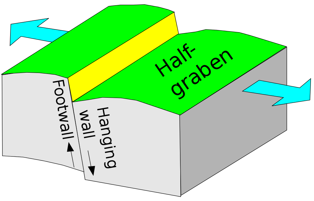
Figure: A half-graben is a geological structure bounded by a fault along one side of its boundaries. Source: Wikipedia.

Review of rock characteristics and classification

Rock composition: minerals, fossils, and other material that make up a rock. Rock composition gives information about the source material for the rock, as well as about processes that occurred during rock formation. In the field, composition is mostly based on identifying the minerals present in a rock. When mineral grains are large, this is relatively easy if you are familiar with a dozen or so common rock-forming minerals. When grains are small, this is difficult but you can often use color to give you general clues about composition.

Rock texture: how the compositional components of a rock are put together. Rock texture gives much information about processes that occurred during rock formation. Train your eye by considering three important observations:

• Is the rock layered? Most sedimentary rocks are layered. Most igneous rocks are not layered. Metamorphic rocks can be layered or unlayered.

• Does the rock have clastic or crystalline texture? In clastic rocks, discrete grains are held together by cementing material between the grains. In crystalline rocks, mineral grains are intergrown so that their grain boundaries interfinger in a jigsaw-puzzle type pattern. N.B. If grains are too small, you can’t make this observation with your naked eye. Most sedimentary rocks are clastic, with the exception of chemical sediments that precipitate out of water. Virtually all igneous and metamorphic rocks are crystalline.

• What is the grain size or range of grain sizes in the rock? Once a rock has been classified by igneous, metamorphic, or sedimentary, further classification is partly based on grain size.

Common sedimentary rocks (mostly clastic, some limestones are crystalline):

Limestone: comprised primarily of the mineral calcite (CaCO₃, applying acid will result in the formation of bubbles (release of CO₂ gas)). Calcite occurs as fossils (shells, etc.) and/or as a chemical sediment formed by precipitating out of water. Dolostone (dolomite) is similar to limestone, but some of the Ca is replaced by Mg. This rock only bubbles if pulverized into small particles before HCl is applied.

Shale: clastic sedimentary rock comprised of clay particles too small to see with the naked eye. Usually a soft, finely-layered rock that looks like compressed mud.

Sandstone: clastic sedimentary rock comprised of sand grains or other sand-sized particles that be been cemented together. Usually gritty to the touch.

Conglomerate: clastic sedimentary rock comprised of poorly-sorted particles of a variety of sizes (clay, sand, pebbles) that have been cemented together.

Common metamorphic rocks (crystalline texture; can be layered or unlayered):

Slate: finely-layered rock which splits parallel to the alignment of fine-grained platy minerals (micas)

Schist: coarser-grained rock with layering defined by parallel alignment of micas

Gneiss: coarse- grained rock characterized bysegregation of minerals into different layers

Marble: metamorphic rock comprised primarily of calcite

Quartzite: metamorphic rock comprised primarily of quartz

Principles of relative dating of geologic structures and events:

Principle of original horizontality of sedimentary layering - sediments are deposited as horizontal layers

Principle of superposition of undeformed sedimentary layering - oldest on the bottom

Principle of igneous intrusions - intrusions must be younger that the rocks they intrude

Principle of cross-cutting relationships – structures must be younger than structures/rock units they cut

Overview of stops and worksheets

Today’s field trip investigates a southeast-to-northwest transect across central New Jersey to investigate the regional geology of this part of the state, and also to fit in into the larger regional geologic history of the North American content, in both time and space. We start at Washington Road very close to Guyot Hall, and then visit two other sites in Princeton before heading northwest to the last two sites along the Delaware River.

Figure: overview of stops during the day.

Here we provide a “cheat sheet” of important characteristics of rocks, common rock names, and a reminder of the principles of relative dating used to decipher the order of geologic events that have affected the area.

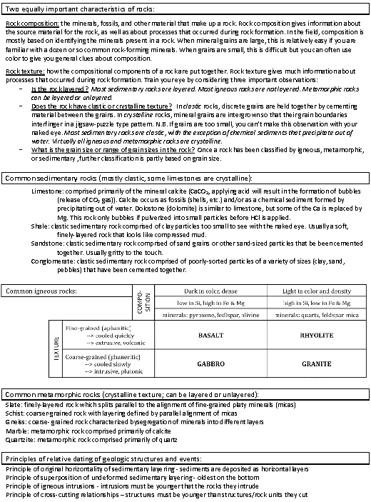
Figure: cheat sheet for rock identification.

This simplified version of the geologic time scale gives the names of the various Eons, Eras, Periods and Epochs of geologic time along with absolute ages of the boundaries between the various Eons, Eras, Periods and Epochs of geologic time. Also noted are important events and in Earth history. Note that the column presented here is distinctly non-linear. For example, the Cenozoic Era takes up 2/5 of the space whereas it only represents ~1.5% of Earth’s age.

Figure: Simplified geological time scale.

An overview of the five stops on the field trip. Both maps cover the same area, with the upper map showing roads, forested areas (in green), and is shaded to reflect the relief of the area. The lower map shows the bedrock geology.

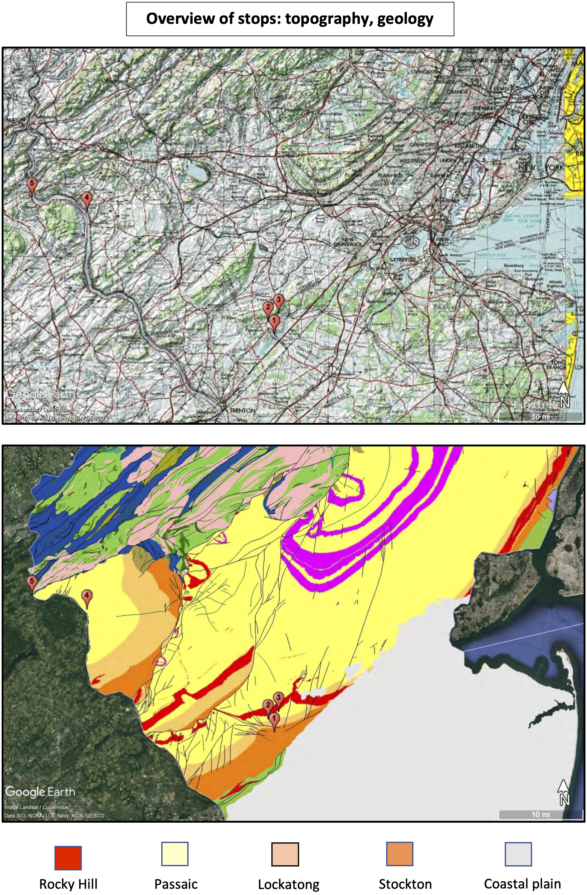
Figure: Overview of stops.

A close-up of the three stops in the Princeton area. Again the two maps cover the same area. Stop 1 is in the Stockton formation. Stop 2 is in the Passaic formation. Stop 3 is at the contact between the Passaic and Rock Hill formations. You should be able to see the correspondence of certain units to certain topographic features.

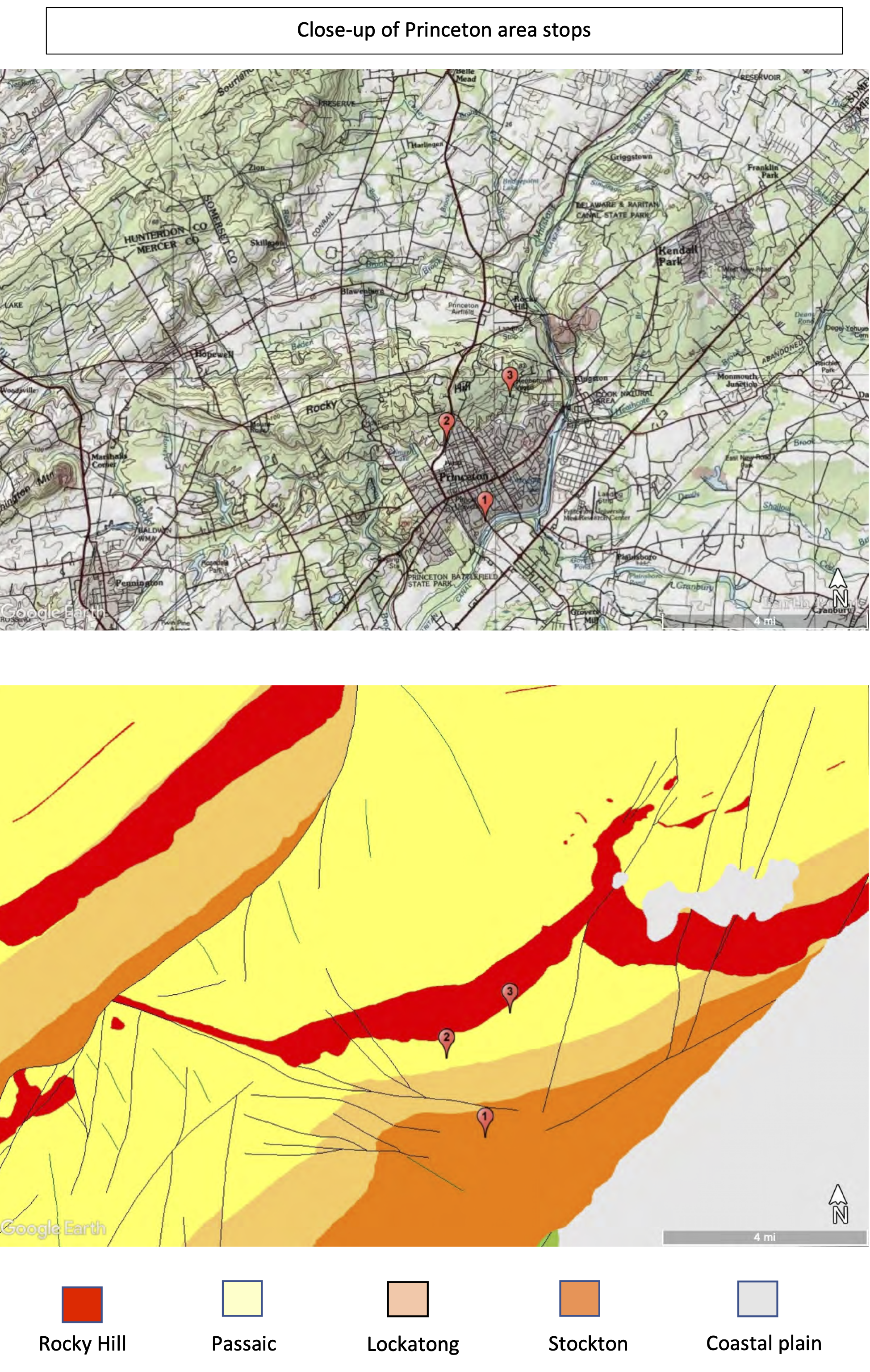
Figure: Overview of stops in the Princeton area.

This is a cross-section running across the trip area from WNW to ESE, with view to the ENE. The position of the five field trips stops is shown, as well as important bedrock structures that we see evidence for on the trip.

Figure: Cross-section across the trip area. The border fault and major internal faults (Flemington-Furlong and Hopewell faults) dip to the southeast; bedding generally dips to the northwest. Post-rift strata pinch out near the edge of the Newark basin. No vertical exaggeration means that the horizontal and vertical scales are the same. Modified from Schlische (1992) and Withjack et al. (2020, 2022). Source: Rutgers University.

Here is the generic worksheet we will be using during the field tirp; you will be given one (hard copy) for each stop to work on during the trip. These will not be collected nor graded, but will form the basis on which you will answer the required questions. Take advantage of the sheets, fill out everything, ask questions, make connections!

Stop 1: Stockton Formation along Washington Rd

Coordinates: (40.341472\(^{\circ}\) N, 74.649972\(^{\circ}\) W), Google Maps: Link

Stop 2: Passaic formation (at Princeton Professional Center)

Coordinates: (40.363704\(^{\circ}\) N, 74.663973\(^{\circ}\) W), Google Maps: Link

Stop 3: Lockatong and Rocky Hill formations (at Herrontown Woods)

Coordinates: (40.376389\(^{\circ}\) N, 74.640472\(^{\circ}\) W), Google Maps: Link

Stop 4: Passaic formation (along Rte 619 north of Frenchtown, NJ)

Coordinates: (40.548944\(^{\circ}\) N, 75.069028\(^{\circ}\) W), Google Maps: Link

Stop 5A and 5B: Passaic and Highlands formations (along Rte 611 south of Riegelsville, PA

Coordinates: (40.572639\(^{\circ}\) N, 75.192583\(^{\circ}\) W), Google Maps: Link

Field Guide

Printed copies of the field guide were distributed during the trip. A slideshow is provided below for quick reference.

TO DO

Question 3.1. We saw four geologic formations today: Stockton, Passaic, Rocky Hill, Highlands. Make a list, with the youngest formation at the top of the list and the others in progressively order of age with the oldest at the bottom. In a few sentences name and describe the rock type(s) of each formation.

Answer:

Question 3.2 Compare/contrast the Passaic formation you saw at Stop 4 (Frenchtown) and Stop 5 (Riegelsville). The rocks are of similar age, and both lie within the Newark rift basin that marks the initial breakup of Pangea. There are no major faults or other deformational structures between them. Yet the rocks at the two stops have different rock types and sedimentary structures. What are the differences, and why are the rocks so different at these two places.

Answer:

Question 3.3 Describe evidence for the “Border Fault” at Stop 5. The fault itself is not exposed. What is the evidence that there is a fault there, and that there is a major amount of displacement along it?

Answer:

Question 3.4 In bullet-list form, summarize the sequential geologic history of the area based on your observations and our discussions during the trip. Your list should include the formation of the various geologic units, igneous events, deformation events, and should end with something like “erosion, exposure and formation of the modern topography.”

Answer: