Earthquake Signals

Part I: Seismicity on Earth

An earthquake is a vibration of Earth caused by the sudden release of energy, usually as an abrupt breaking of rock along planar fractures called faults. An earthquake initiates at its hypocenter or focus at some depth below the land surface or sea floor. The epicenter of the earthquake is defined as the point on the Earth’s surface above where the earthquake initiated.

But only rocks that are relatively cold and brittle (the Earth’s lithosphere) can be broken in earthquakes. Rocks that are hot and ductile (e.g. the Earth’s asthenosphere) will deform without breaking, and therefore do not produce earthquakes. By observing where earthquakes occur, both horizontally and with depth, we can learn where stress is concentrated and infer the material properties of the Earth.

In this section, we will examine the distribution of earthquakes. You will notice that most of them are near plate boundaries. Each type of plate boundaries has a unique moving pattern shown in the image below. Keep this in mind when you look at the earthquake epicenter plot later in this section.

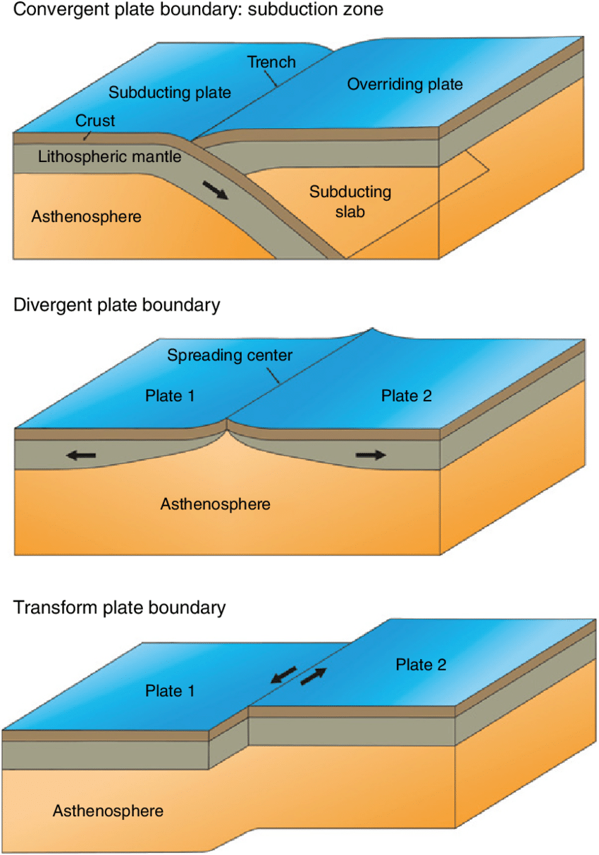
Image: Three major types of plate boundaries.

Review

Feel free to adjust the filter parameters in the cell below to have more or less earthquakes on the map. You may hover the dots to get the information of the earthquakes. The colors of the lines indicate the type of plate boundaries: Red is a Trench, Green is a Transform, and Blue is a Ridge boundary.

Question Examine the regions on and around Earth’s ocean ridges and ocean trenches. Both the spatial distribution and the depths of earthquakes associated with each are different. Describe/illustrate these differences between earthquake associated with ridges and earthquakes associated with trenches.

Answer:

Question. Using earthquake depths as evidence, discuss whether the Earth’s lithosphere is thicker at ridges or at trenches.

Answer:

Part II: Seismic stations, seismographs, and seismograms

Seismographs are instruments at seismic stations that measure ground motion. The data is displayed as seismograms. This data is of fundamental importance to the geosciences. By studying earthquake-generated ground motion we can learn about 1) the nature of the earthquake itself (the source of the motion) and 2) the material the earthquake waves travel through (Earth’s interior). This is because the observed vibration (in the time domain t) is the result of the effects of earthquake source, interior structure and how the instrument senses the vibration. These effects can be most easily modeled by considering each frequency (\(\omega\)) of the waveform in turn, and using their products (i.e. frequency-domain convolution per mathematical definition) to derive the waveform.

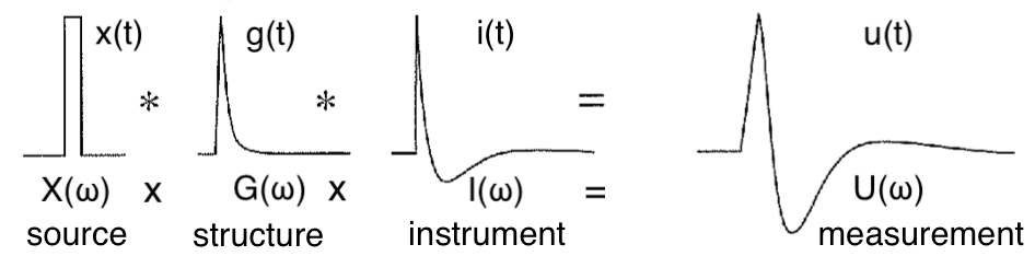
Figure: Relationship between measurement and contribution from instrument, structure and source.

The United States Geologic Survey estimates that several million earthquakes occur each year. Many go undetected because they hit remote areas without good seismic station coverage, or have very small magnitudes. But various seismic networks locate something like 20,000 earthquakes a year. We will focus on two large earthquakes since they caused the whole Earth to ring like a bell, causing waveforms to be recorded at various stations well above the noise level of the instrument.

Tohoku earthquake USGS Link

The March 11, 2011, M 9.1 Tohoku earthquake, which occurred near the northeast coast of Honshu, Japan, on the subduction zone plate boundary between the Pacific and North America plates. The location, depth (about 25 km), and focal mechanism solutions of the March 11th earthquake are consistent with the event having occurred on the subduction zone plate boundary. Modeling of the rupture of this earthquake indicates that the fault moved as much as 50–60 m, and slipped over an area approximately 400 km long (along strike) by 150 km wide (in the down-dip direction). The Japan Trench subduction zone has hosted nine events of \(m_w\) 7+ since 1973.

The focal mechanisms that are usually given to convey this configuration are a way of plotting the three dimensional fault information in two dimensions (they’re lower hemisphere stereographic projections). The figure below is an attempt to show how a simple block model of the first motions of 5 common types of earthquake look when projected onto a lower hemisphere, and then when the pattern on that focal sphere is projected onto the horizontal to produce a 2D focal mechanism.

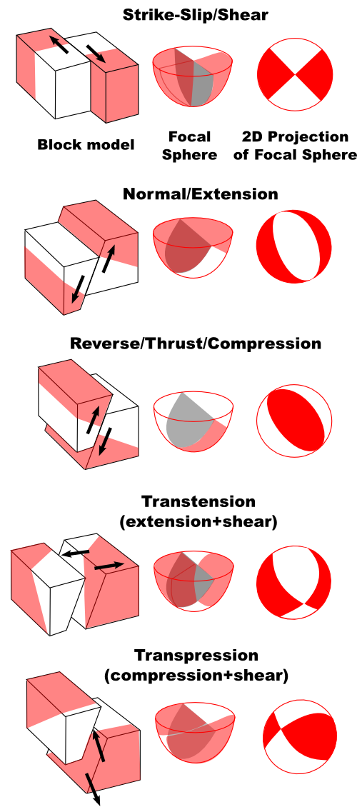
Figure: Types of faulting and their expression as focal mechanism of the earthquake.

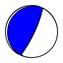
The Global Centroid-Moment-Tensor (CMT) Project has measured the moment tensors of all earthquakes with magntiudes \(m_w\) 5.5+ since 1976. The CMT project has been continuously funded by the National Science Foundation since its inception. Let us read the CMT solution of the Tohoku earthquake in the CMTSOLUTION format, available from their webpage.

TO DO

Question Based on the beachball focal mechanism above, what type of faulting caused the Tohoku earthquake? Was the fault shallowly dipping at a low angle from the surface (dip < 30\(^{\circ}\)) or steeply dipping at a high angle (dip > 60\(^{\circ}\))? Which plate was the overriding plate?

Answer:

Section A: Vibrations at a single station

Modern seismometers measure ground motion in three mutually perpendicular directions:

• North-South (LHN or BHN component). This records the north-south horizontal component of vibration. “Up” on this graph means the ground moved north. “Down” on this graph means the ground moved south.

• East-West (LHE or BHE component). This records the east-west horizontal component of vibration. “Up” on this graph means the ground moved east. “Down” on this graph means the ground moved west.

• Vertical (LHZ or BHZ component). This records the vertical component of vibration. “Up” on this graph the means the ground moved up. “Down” on this graph means the ground moved down.

The prefix (L-long period, or B-broadband) indicates the sampling rate of seismic data stream. When we wish to analyse signals that are finely spaced, we use the broadband data steam (i.e. think of Nyquist frequency). Sometimes, the horizontal orientations of the sensor in the instrument are not perfectly aligned with the N-S and E-W directions, even if the vertical component is perfectly aligned. In these cases, the horizontal components are denoted as LH1 and LH2 (or BH1 and BH2). We typically analyze the motion along the propagation direction of the wavefront, which gives us clearer information on individual seismic phases (as you will see below). Note that finding the propagation direction from earthquake to a station requires the coordinates and depth of the hypocenter, as denoted by the CMT focal mechanism above.

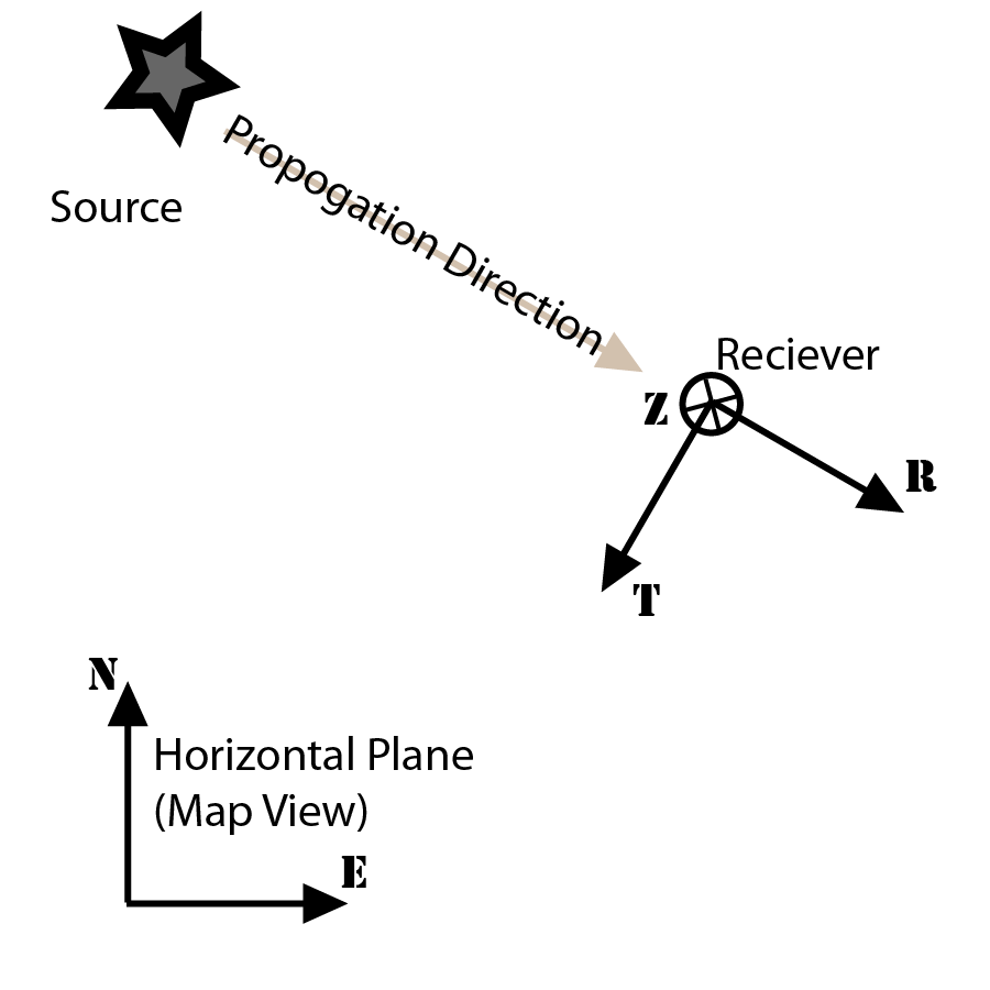
Figure: Rotation of vibrations recorded on a seismogram to radial, transverse and vertical components along the propagation direction.

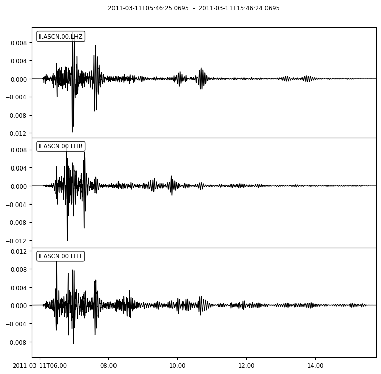
Let us perform this calculation for the vibrations recorded on the long-period components at Ascension Island (station code: ASCN) in the South Atlantic Ocean from the Tohoku earthquake.

3 Trace(s) in Stream:
II.ASCN.00.LH1 | 2011-03-11T05:46:25.069500Z - 2011-03-11T15:46:24.069500Z | 1.0 Hz, 36000 samples
II.ASCN.00.LH2 | 2011-03-11T05:46:25.069500Z - 2011-03-11T15:46:24.069500Z | 1.0 Hz, 36000 samples
II.ASCN.00.LHZ | 2011-03-11T05:46:25.069500Z - 2011-03-11T15:46:24.069500Z | 1.0 Hz, 36000 samples

We also wish to focus on vibrations in the period range 20-200 seconds to start with. This done by band-pass filtering the seismogram below:

Section B: Horizontal versus Vertical Motions

Task I: At a single station

TO DO

Question Identify the first seismic wave arrival at your station on the Z component. This is the first P-wave. Note that you should consider when the seismograph first starts to respond to the P-wave – i.e., the “shoulder” of the wave, or where trace starts to climb or fall towards the first peak or trough. Report your P-wave travel time pick in minutes and seconds.

Answer:

Question Identify the first S-wave arrival at your station. Hint: how would the relative horizontal vs. vertical motion differ for an S wave compared to a P wave? There may also be a change in wavelength and/or amplitude; S-waves look ‘different” than P-waves. But there is likely more uncertainty about when to “pick” the arrival time of the first S-wave. This is because by this time, the station is still responding to the passage of P and other waves; and the S-waves are superimposed on these other waves. This is part of the “art” of seismology – and also partly why we use data from many stations to analyze seismic waves. Report your S-wave travel time pick in minutes and seconds.

Answer:

Question Identify the surface waves on the seismogram. These are the waves with the strongest vibrations (largest amplitudes). Provide your travel time picks for the Rayleigh and Love wave packets on Z and T components, respectively. Note: Picking a travel time of a surface wave is complicated and depends strongly on the frequency of the surface wave, due to a property called dispersion. For this task, simply report the time of the first shoulder from the left (earliest in time). Which of the two waves (Love or Rayleigh) is arriving sooner at the station?

Answer:

Task II: Record Section of the USArray Transportable Array

A single seismometer can give us some information about the earthquake and interior structure. In fact, this is the idea behind deploying a seismometer on the Moon and Mars. However, arrays of seismometer can provide unprecedented insights into geological processes.

USArray is a 15-year program to place a dense network of permanent and portable seismographs across the continental United States. The seismographs record local, regional, and distant (teleseismic) earthquakes. This mega-project is funded by the US National Science Foundation and we will use data from a part of this project called the Transportable Array.

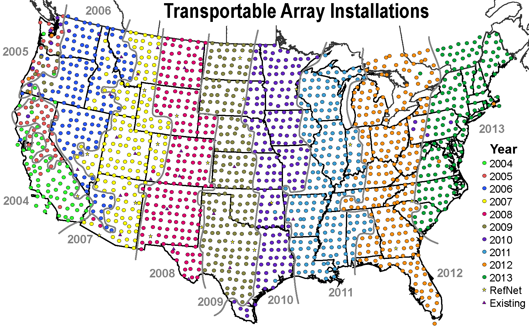
Figure: Installation plan of the transportable array of USArray.

USArray has a large traveling network of 400 high-quality, portable seismographs that are being placed in temporary sites across the United States in a rolling fashion. Station spacing is ~70 km (42 mi). Transportable Array data are extremely useful for mapping the structure of Earth’s uppermost 70 km. The array was initially deployed in the westernmost United States. Unless adopted and made into a permanent installation, after 18-24 months, each instrument is picked up and moved to the next carefully spaced array location to the east. When completed, over 2000 locations will have been occupied during this program.

Note that since we are looking at the data from Tohoku earthquake in 2011, we are using data from the Transportable Array as it was installed at that time. This means the stations that we are analyzing lie on a grid from Michigan to Louisiana.

TO DO

Question The record sections above show data from the first hour after the earthquake origin time on the Z and T components. Zoom into any distance range 10 degrees in width, and download the image as png from the options (top right). Draw a line with a red pen where you see the P wave (on the Z component) and S wave (on the T component). Find slope of this curve and report this as the speed of the P and S wave (in m/s). Are the slopes expected to vary with distance? If so, why? Hint: You can assume that 1 degree equals 111.1949 km on average. Attach the annotated image with the assignment.

Answer:

Part 2: Waveforms at different period bands

Next, we will evaluate if we can glean more information by analyzing waveforms at other period bands. As you will see, there is a plethora of information in these seismograms at various period/frequency bands. Let us look at the vertical (Z) component from the US Transportable Array at two period bands (5-40 seconds vs 20-100 seconds).

TO DO

Question The record sections above show data from the first hour after the earthquake origin time on the Z component for data filtered at two period bands (5-40 seconds vs 20-100 seconds). Do you see any phases that are more prominent in one period band or the other? Annotate this phase by zooming into any distance range 10 degrees in width, and downloading the image as png from the options (top right). Attach the annotated image with the assignment.

Answer:

Part 3: Spectrum of Vibrations

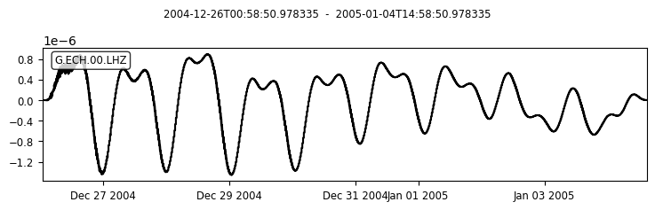
To complete the illustration of time versus frequency plots (a normal signal versus it’s spectrum), here is a seismic signal (ground motion caused by an earthquake). The time series is a complicated looking signal. In fact, this signal can be described as a combination of a very large number of sinusoids, all with amplitudes as shown in the spectrum graph.

2004 Sumatra - Andaman Islands Earthquake USGS Link

The devastating M 9.1 earthquake off the west coast of northern Sumatra on December 26, 2004, occurred as the result of thrust faulting on the interface of the India plate and the Burma microplate. In a period of minutes, the faulting released elastic strains that had accumulated for centuries from ongoing subduction of the India plate beneath the overriding Burma microplate.

Since this earthquake was so large, it was able to ring the Earth like a bell, causing vibrational normal modes or standing waves. Let us look at the data from this earthquake recorded at Echery - Sainte Marie aux Mines, France.

TO DO

Question Report the approximate frequencies that you observe on the spectrum here. Identify the lowest frequency (longest period) normal mode and describe how it deforms the Earth.

Answer:

TO DO

Question Seismometer are so sensitive that they also record vibrations due to tides in the solid Earth. An example is seen in the spectrum above. Report the two frequencies. Convert to minutes/hours and comment on the forces causing these longer period vibrations (compared to seismic waves).

Answer: